Introduction to GraphSAGE
Graph SAmple and aggreGatE
Overview and Motivation
Topics
The goal of this porption lecture
- Understand what problem GraphSAGE was invented to solve
- Understand the three step recipe: sample, aggregate, update
- Walk a complete numerical example from raw features all the way to a loss value
- Build a working model in PyTorch Geometric
What you should already have
- Comfort with vectors and matrix multiplication
- A rough idea of what a neural network layer does
- Familiarity with gradient descent and cross entropy loss
What we will not cover
- Formal proofs of expressive power
- Heterogeneous graphs, temporal graphs, or graph level prediction
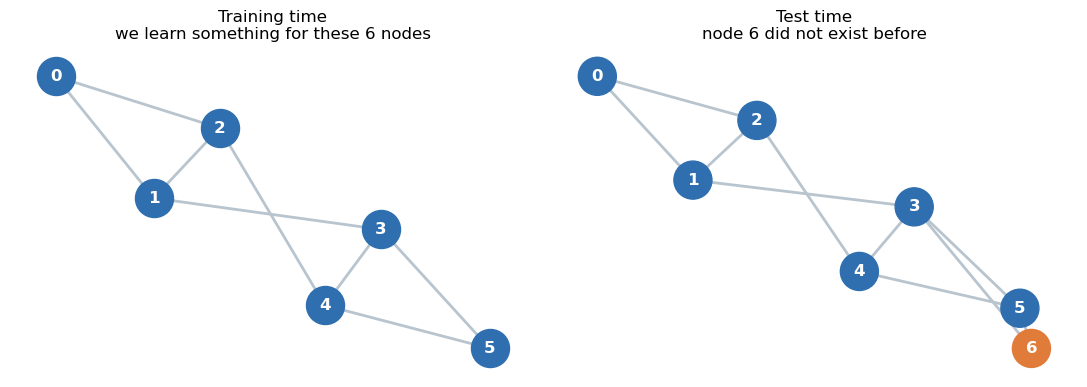
Recall: Transductive vs. Inductive Learning
- Transductive Learning
- Learns an embedding for each node directly (creates a lookup table)
- Cannot generate embeddings for new/unseen nodes
- Inductive Learning
- Learns a function to generate embeddings based on node features and structure
- Can compute representations for new/unseen nodes without retraining
The Problem with Lookup Table Methods
Transductive approaches:
- Learn a unique embedding for each node—stored in a lookup table (e.g., DeepWalk, node2vec) - The model is ultimately just a matrix \(Z\) (one row per node) - Training = directly updating these node-specific rows - Again, think \(T-SNE\) flavor, where we retrain the embedding for each new points
Limitations:
- No vector exists for new nodes; cannot embed them - Only solution: retrain or re-optimize on the whole graph - Parameter count scales linearly with node count
Real-world impact:
- Large dynamic graphs (Reddit posts, Pinterest pins, fraud accounts) constantly add new nodes - Constant retraining is infeasible and inefficient
The Two Problems GraphSAGE Solves
- Introduced by Hamilton, Ying, Leskovec (2017) to address:
1. New Nodes (Inductive Learning)
- Embed unseen nodes without retraining the model
2. Scalability
- Full-graph methods can’t handle massive graphs in memory
- Necessary for dynamic graphs (e.g., social platforms, recommendation systems)
Key idea
- Learn a shared function (neural aggregator) instead of per-node embeddings
- Parameters are function weights, not node vectors
- Applies to any node—seen or unseen
- Operates on local neighborhoods; efficiently runs in mini-batches
General overview of the method
Recall; Message Passing Formalism
Node representations are updated by exchanging information through edges
Each node aggregates messages from its local neighbors
General message passing update:- For target node \(v\):
- Gather: collect representations from neighbors \(u \in \mathcal{N}(v)\)
- Aggregate: combine neighbor information (e.g., mean, sum, LSTM)
- Update: merge aggregated message with \(v\)’s existing representation
- For target node \(v\):
Framework underlies GCN, GAT, GraphSAGE, and many other GNNs
Big picture: Sample, Aggregate, Update
The name GraphSAGE comes from SAmple and aggreGATE. Every layer does three things for a target node \(v\).
Sample: Select a fixed number (e.g., 10) of neighbors for node \(v\) uniformly at random; ignore others.
Aggregate: Merge sampled neighbor vectors into one summary—commonly by elementwise mean.
Update: Combine the neighbor summary with \(v\)’s vector, apply a learned weight matrix and nonlinearity.
Stacking layers allows information to propagate from further neighborhoods.
Summary: A node’s updated embedding is a learnable blend of its own features and aggregated knowledge from its sampled neighbors.
Step 1: Sample the Neighborhood
Importance of Sampling
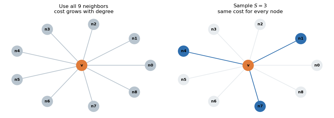
Problems with using all neighbors
- Real graphs: highly variable node degrees
- Example: most Twitter users follow hundreds; celebrities, millions
- Large-degree nodes in a batch can cause memory spikes
Advantages of fixed-size sampling
- Constant per-node cost—predictable batch sizes
- Memory/compute become tunable hyperparameters, not data-dependent
- Adds randomness, acting as regularization (like dropout)
Practical points
- Neighbors are sampled uniformly from \(\mathcal{N}(v)\)
- If \(|\mathcal{N}(v)| < S\), sample with replacement to always get \(S\)
- Sampling is redone at each training step, covering the full neighborhood across epochs
Key intuition: Sampling provides a Monte Carlo estimate of aggregating all neighbors: noisy short term, accurate on average.
Step 2: Aggregate
- Given \(S\) sampled neighbor vectors, aggregate them into a single summary vector.
- Key requirement: Aggregation must be permutation invariant (order does not affect result).
- Neighborhood is a set, not an ordered list.
- No meaningful order among neighbors.
- Order-dependent functions yield inconsistent outputs for the same graph.
The mean aggregator
\[h_{\mathcal{N}(v)}^{k} = \frac{1}{|S_v|} \sum_{u \in S_v} h_u^{k-1}\]
Read this as: take the \(S\) sampled neighbor vectors from the previous layer and average them componentwise.
A tiny numeric check
If the three sampled neighbors have vectors \([1, 0]\), \([0, 2]\), and \([2, 1]\), then
\[h_{\mathcal{N}(v)} = \frac{1}{3}\left([1,0] + [0,2] + [2,1]\right) = \frac{1}{3}[3, 3] = [1, 1]\]
Step 3: Update
The Equation for a single GraphSAGE Layer
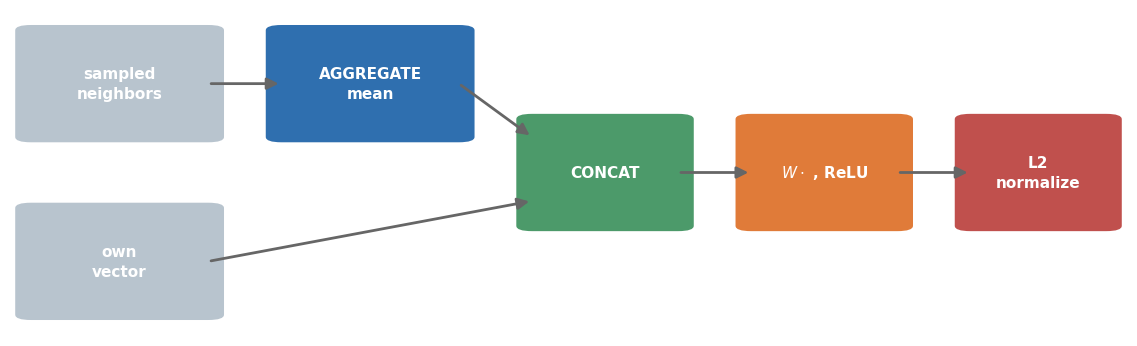
Putting the three steps together, one GraphSAGE layer \(k\) computes:
\[h_{\mathcal{N}(v)}^{k} = \text{AGGREGATE}_k\left(\{\, h_u^{k-1} : u \in S_v \,\}\right)\]
\[h_v^{k} = \sigma\left( W^{k} \cdot \text{CONCAT}\left(h_v^{k-1},\; h_{\mathcal{N}(v)}^{k}\right) \right)\]
\[h_v^{k} \leftarrow \frac{h_v^{k}}{\lVert h_v^{k} \rVert_2}\]
Meaning of the symbols
- \(h_v^{k}\) is node \(v\)’s vector after \(k\) layers, and \(h_v^{0} = x_v\) is the raw feature vector
- \(\sigma\) is a nonlinearity, normally ReLU
- \(W^{k}\) is a learned weight matrix shared by every node in the graph
- \(\lVert \cdot \rVert_2\) is the Euclidean length, so the last line rescales the vector to length 1
Why concatenate, not just average?
- Keeps the node’s own features separate from neighbors’
- Lets the weight matrix treat “me” and “neighbors” differently
- If combined into a mean, the model cannot distinguish the two sources
Why L2 Normalization?
- Rescales embeddings to unit length—removes magnitude, preserves direction.
- Controls for node degree: prevents high-degree nodes from having outsized embedding norms.
- Stabilizes activations across stacked layers, improving optimization.
- Ensures dot product between embeddings gives cosine similarity—enables meaningful similarity search.
Example:
If \(z = [3, 4]\), then
\[\|z\|_2 = 5,\;\;\; \hat{z} = \left[\frac{3}{5}, \frac{4}{5}\right] = [0.6,\;0.8]\]
Direction unchanged; length is now 1.
Stacking Layers: Fanning effect from sampling
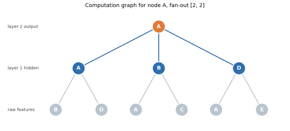
- To compute node A’s layer 2 embedding:
- Need layer 1 embeddings for A and sampled neighbors B, D
- Each layer 1 embedding depends on the raw features of its own sampled neighbors
- The process forms a small computation tree, traced backward from the target node
Interpretation - Embedding at layer \(K\) draws from nodes up to \(K\) hops away (receptive field)
Computation Cost - With fan out \([S_1, S_2, \dots, S_K]\), number of nodes per tree: \[ 1 + S_1 + S_1S_2 + \dots \approx \prod_{k=1}^K S_k \] - Where \(S_k\) is the number of neighbors sampled at layer \(k\) - Example: Fan outs - \([10, 10]\) ≈ 100 nodes per target - \([10, 10, 10]\) ≈ 1000 - Paper suggests \(K=2\), \(S_1 \cdot S_2 \leq 500\)
Depth tradeoff - More layers = wider reach, but too much depth (\(>2\)–\(3\)) causes oversmoothing: all embeddings converge and lose distinction
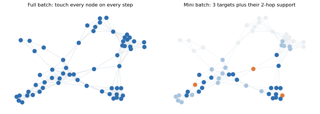
Why Mini-Batching Matters
- Full graph methods:
- Load entire graph and features in memory
- Recompute all node embeddings each step
- Impractical for large graphs
- GraphSAGE:
- Sample a batch of \(B\) target nodes
- For each, sample their \(K\)-hop neighborhoods (fan out \([S_1, ..., S_K]\))
- Batch size is proportional to \(B \cdot \prod_k S_k\), independent of total graph size
- Compute loss and backprop on targets only
- Consequences:
- Memory and compute scale with batch size, not graph size
- Graph can be kept on disk or in distributed storage
- Training scales with labeled data, not total nodes
- Inference:
- Use full neighborhoods at prediction time; no need for sampling
Sampling with Limited Neighbors
- \(S\): sample size (fanout); \(N(v)\): neighbor set of node \(v\)
- If \(|N(v)| < S\), two sampling options:
- With replacement (
replace=True):- Sample \(S\) nodes, allowing repeats
- Fixed output size; original GraphSAGE approach; efficient for GPU batching
- Without replacement (
replace=False):- Return all \(|N(v)|\) neighbors (may be fewer than \(S\))
- Default in PyG/DGL; produces variable/neighborhood sizes; requires padding and masking
- With replacement (
- Special cases:
- Isolated nodes (\(|N(v)| = 0\)): use self-loop or zero vector for aggregation
- With replacement: consistent shapes, but duplicated neighbors
Alternative Aggregators
- Key hyperparameter; classic options:
- Mean
\[\text{AGG} = \frac{1}{|S_v|}\sum_{u \in S_v} h_u\]- Simple, robust default
- Ignores neighbor counts
- Max Pooling
\[\text{AGG} = \max\left(\left\{\, \sigma(W_{\text{pool}} h_u + b) : u \in S_v \,\right\}\right)\]- Passes neighbors through a small network, then elementwise max
- Effective to detect if any neighbor has a feature
- More parameters; may overfit
- LSTM
- Sequentially aggregates neighbors (random order each batch)
- Highest capacity; not fully permutation invariant
- Mean
- Guidance: Use mean by default; try max pooling if outlier neighbors are important.
Key Hyperparameters
- Layers (\(K\)): Usually 2–3; more layers risk oversmoothing.
- Fan out \([S_1, S_2]\): Typical values \([25,10]\) or \([10,5]\); higher values reduce variance but increase compute. Keep total under a few hundred.
- Hidden dimension: 64–256; larger = better for rich graphs, prone to overfit on small graphs.
- Aggregator: Mean (default), or max pooling for “any neighbor” detection.
- Neural network settings: Learning rate ≈ \(0.01\) (Adam), dropout ≈ 0.5, weight decay ≈ \(5 \times 10^{-4}\) (small graphs).
- Batch size: Affects throughput/memory; interacts with fan out.
Why GraphSAGE Generalizes to Unseen Nodes
- Stores only weight matrices \(W^{1}, \dots, W^{K}\); nothing tied to node IDs
- Parameter count does not depend on number of nodes \(|V|\)
- Embedding a new node \(v\) requires:
- Its feature vector \(x_v\)
- Its edges (to sample neighbors)
- Same forward pass, same weights—no retraining needed
- Learns rules based on neighbor features, not node identity
- Generalizes: can compute embeddings for unseen nodes if they have features and edges
- Limitation: New nodes must have features in the same space; no features/edges ⇒ not supported
Why GraphSAGE Is Inductive, GCN Is Transductive
- Key distinction:
- GCN learns fixed node embeddings.
- GraphSAGE learns shared aggregation functions.
- GCN:
- Layer: \(H^{(l+1)} = \sigma(\tilde{D}^{-1/2}\tilde{A}\tilde{D}^{-1/2} H^{(l)} W^{(l)})\)
- Relies on full adjacency matrix; each node’s embedding is position-specific.
- Adding nodes requires recomputing all representations (since \(\tilde{A}\) changes).
- GraphSAGE:
- Layer: \(h_v^{(l+1)} = \sigma(W^{(l)} \cdot \text{concat}(h_v^{(l)}, \text{agg}(\{h_u^{(l)} : u \in N(v)\})))\)
- Learns a function; same parameters applied to any node with its features and neighbors.
- Generalization advantage:
- Embeddings generated on demand from features, not tied to node identity.
- Scales to unseen nodes/graphs at inference–no retraining if features and edges are available.
- Minibatch training enabled by local neighbor sampling rather than full adjacency.
Toy Example calculation:
Problem Setup
The graph
| Node | Feature \(x_v\) | Neighbors |
|---|---|---|
| A | \([1, 0]\) | B, C, D |
| B | \([0, 1]\) | A, C |
| C | \([1, 1]\) | A, B, E |
| D | \([2, 0]\) | A, E |
| E | \([0, 2]\) | C, D, F |
| F | \([1, 2]\) | E |
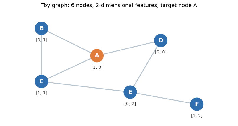
Our toy Architecture
Consider the calculation for node A.
The model
- Two GraphSAGE layers, mean aggregator, sample size \(S = 2\) at both hops
- Both layers map 2 dimensions in to 2 dimensions out, so each \(W\) is \(2 \times 4\)
- ReLU nonlinearity, then L2 normalization
- A linear classifier head on top, then softmax and cross entropy
- Binary classification, and node A’s true label is \(y_A = 1\)
The weights (pretend these came from an earlier training step)
\[W^{1} = \begin{bmatrix} 1 & 1 & 1 & 0 \\ 0 & 1 & 0 & 1 \end{bmatrix} \qquad W^{2} = \begin{bmatrix} 1 & 0 & 1 & 0 \\ 0 & 1 & 0 & 1 \end{bmatrix} \qquad W^{\text{out}} = \begin{bmatrix} 2 & -1 \\ -1 & 2 \end{bmatrix}\]
Biases are zero throughout, to keep the arithmetic readable.
Step 0: Sampling the Computation Graph
- Goal: Identify minimal subgraph required to compute node A’s output, working backwards from A.
- Hop 1:
- A’s neighbors: \(\mathcal{N}(A) = \{B, C, D\}\)
- Randomly sample \(S=2\): example \(\{B, D\}\)
- Hop 2:
- \(\mathcal{N}(B) = \{A, C\}\) → use both
- \(\mathcal{N}(D) = \{A, E\}\) → use both
- For A’s own vector, reuse sampled \(\{B, D\}\)
- Touched nodes: \(\{A, B, C, D, E\}\)
(F is not reached; only 2 hops from A) - Compute sequentially:
- Layer 1: \(h_A^{1}\), \(h_B^{1}\), \(h_D^{1}\)
- Layer 2: \(h_A^{2}\)
- Output: logits, softmax, loss
Step 1: Layer 1 for Node B
Recall the layer equation, and remember \(h_v^{0} = x_v\).
Aggregate. B’s sampled neighbors are A and C.
\[h_{\mathcal{N}(B)}^{1} = \tfrac{1}{2}\left( [1, 0] + [1, 1] \right) = \tfrac{1}{2}[2, 1] = [1,\; 0.5]\]
Concatenate B’s own feature with that summary:
\[\text{CONCAT}\left(h_B^{0},\, h_{\mathcal{N}(B)}^{1}\right) = [\,0,\; 1,\; 1,\; 0.5\,]\]
Multiply by \(W^{1}\), one output component at a time:
\[z_1 = (1)(0) + (1)(1) + (1)(1) + (0)(0.5) = 2\] \[z_2 = (0)(0) + (1)(1) + (0)(1) + (1)(0.5) = 1.5\]
so \(z = [2,\; 1.5]\).
ReLU. Both entries are positive, so nothing changes: \([2,\; 1.5]\).
L2 normalize.
\[\lVert z \rVert_2 = \sqrt{2^2 + 1.5^2} = \sqrt{6.25} = 2.5 \qquad\Rightarrow\qquad h_B^{1} = [0.8,\; 0.6]\]
Step 2: Layer 1 for Nodes D and A
Same recipe, different rows. Nothing new to learn here, so we go quickly.
Node D, sampled neighbors A and E:
- Aggregate: \(\tfrac{1}{2}([1,0] + [0,2]) = [0.5,\; 1]\)
- Concat: \([\,2,\; 0,\; 0.5,\; 1\,]\)
- \(W^{1}\): \(z_1 = 2 + 0 + 0.5 + 0 = 2.5\), and \(z_2 = 0 + 0 + 0 + 1 = 1\)
- ReLU: \([2.5,\; 1]\)
- Norm: \(\sqrt{6.25 + 1} = \sqrt{7.25} = 2.693\), so \(h_D^{1} = [0.928,\; 0.371]\)
Node A, sampled neighbors B and D:
- Aggregate: \(\tfrac{1}{2}([0,1] + [2,0]) = [1,\; 0.5]\)
- Concat: \([\,1,\; 0,\; 1,\; 0.5\,]\)
- \(W^{1}\): \(z_1 = 1 + 0 + 1 + 0 = 2\), and \(z_2 = 0 + 0 + 0 + 0.5 = 0.5\)
- ReLU: \([2,\; 0.5]\)
- Norm: \(\sqrt{4 + 0.25} = \sqrt{4.25} = 2.062\), so \(h_A^{1} = [0.970,\; 0.243]\)
Where we stand
| Node | \(h^{0}\) | \(h^{1}\) |
|---|---|---|
| A | \([1, 0]\) | \([0.970,\; 0.243]\) |
| B | \([0, 1]\) | \([0.800,\; 0.600]\) |
| D | \([2, 0]\) | \([0.928,\; 0.371]\) |
Notice all three layer 1 vectors have length 1, as promised.
Step 3: Layer 2 for Node A
Inputs: Use layer 1 vectors.
Aggregate neighbors (B, D) in layer 1: \[h_{\mathcal{N}(A)}^{2} = \tfrac{1}{2}\left([0.970, 0.243] + [0.928, 0.371]\right) = [0.864,\; 0.486]\]
Concatenate with A’s layer 1: \[[\,0.970,\; 0.243,\; 0.864,\; 0.486\,]\]
Linear transform (\(W^2\)): \[z_1 = 0.970 + 0.864 = 1.834,\quad z_2 = 0.243 + 0.486 = 0.728\]
ReLU: output unchanged.
L2 normalize: \[\lVert z \rVert_2 = \sqrt{1.834^2 + 0.728^2} = 1.974\] \[h_A^{2} = [0.929,\; 0.369]\]
Final embedding for A captures info from B/D directly, C/E indirectly.
Step 4: Classifier Head and Softmax
The embedding is not a prediction yet. We attach a linear head.
Logits
\[\text{logits} = W^{\text{out}} z_A = \begin{bmatrix} 2 & -1 \\ -1 & 2 \end{bmatrix} \begin{bmatrix} 0.929 \\ 0.369 \end{bmatrix}\]
\[\ell_0 = (2)(0.929) + (-1)(0.369) = 1.858 - 0.369 = 1.490\] \[\ell_1 = (-1)(0.929) + (2)(0.369) = -0.929 + 0.738 = -0.191\]
Softmax turns logits into probabilities:
\[p_c = \frac{e^{\ell_c}}{\sum_j e^{\ell_j}}\]
\[e^{1.490} = 4.436, \qquad e^{-0.191} = 0.826, \qquad \text{sum} = 5.262\]
\[p_0 = \frac{4.436}{5.262} = 0.843, \qquad p_1 = \frac{0.826}{5.262} = 0.157\]
The model’s answer
It says class 0 with 84.3 percent confidence.
Step 5: The Loss
- Node A: true label \(y_A = 1\), model predicts class 0 with high confidence
- Cross-entropy loss:
- \[L = -\log p_{y} = -\log(0.157) = 1.852\]
- Interpretation:
- \(L = 0\) for perfect prediction (\(p_y = 1\))
- \(L = 0.693\) for random guess (\(p_y = 0.5\))
- \(L = 1.852\) is “confidently wrong”
- Gradient signal (softmax + cross-entropy):
- \[\frac{\partial L}{\partial \ell} = p - \text{onehot}(y) = [0.843,\; 0.157] - [0,\; 1] = [0.843,\, -0.843]\]
- Push logit 0 down, logit 1 up (strongly)
Step 6: Backward Pass & Updates
- Gradients flow backwards through the computation graph:
- \(\partial L / \partial \ell\) updates \(W^{\text{out}}\), sends gradient to \(z_A\)
- Gradient passes through layer 2 (norm, ReLU) into \(W^{2}\) and the concatenated vector
- Concatenation splits gradient: half to \(h_A^{1}\), half to the neighbor mean
- Mean splits evenly to \(h_B^{1}\) and \(h_D^{1}\)
- These propagate back through layer 1 and \(W^{1}\)
- Only \(W^{1}\), \(W^{2}\), and the head are updated; node embeddings are not stored or learned directly
- The same weight matrices process all nodes—learning a procedure that generalizes to unseen nodes
Technical considerations
Supervised Training
If you have labels, this is ordinary supervised learning with an unusual forward pass.
The setup
- Each labeled node \(v\) has a target \(y_v\), for example a paper’s subject area
- Run the forward pass to get \(z_v\), apply a head, compare to \(y_v\)
The loss
\[L = \frac{1}{|V_{\text{train}}|} \sum_{v \in V_{\text{train}}} \text{CrossEntropy}\left(\text{softmax}(W^{\text{out}} z_v),\; y_v\right)\]
Common node level tasks
- Node classification: what category is this paper, is this account fraudulent
- Node regression: predict a continuous quantity per node
- Link prediction: score a candidate edge as \(\sigma(z_u^{\top} z_v)\)
One thing to watch
Labels are often scarce. Cora, the dataset we use later, has 2708 nodes but only 140 labeled training nodes. The graph structure is doing most of the work.
Mini Batching on a Huge Graph
Practical concerns
- Sampling variance
- Small fan-out → noisy embeddings, erratic validation curves
- Solutions: increase fan-out, or average multiple inference samples
- Oversmoothing
- Too many layers → embeddings collapse to a single vector; low training accuracy
- Solutions: use 2–3 layers or add residual connections
- Featureless nodes
- GraphSAGE requires node features (\(x_v\))
- If missing: substitute degree, node type, or structural summaries
- One-hot identity features make the model transductive
- Feature scaling
- Averaging neighbors distorts unscaled features
- Normalize features before training
- Isolated nodes
- No neighbors = empty neighborhood; fallback is to use only the node’s features
Comparison to other models
GraphSAGE Next to Its Neighbors
| Learns | Neighborhood | Scales by sampling | Inductive | |
|---|---|---|---|---|
| node2vec | one vector per node | random walks | no | no |
| GCN | weight matrices | all neighbors, degree weighted | not as originally posed | architecture yes, standard training no |
| GraphSAGE | weight matrices | fixed size random sample | yes | yes |
| GAT | weights plus attention | all neighbors, learned weights | possible, with care | yes |
How to read the table:
- node2vec: Lookup table; works well for static graphs, can’t generalize to unseen nodes.
- GCN: Aggregates all neighbors with fixed weights; processes the entire graph at once, architecture is generalizable.
- GraphSAGE: Learns neighbor aggregation with sampling, enabling scalability and inductive capability.
- GAT: Learns attention weights for neighbors; more expressive, can combine sampling and attention.
Model progression: - GCN introduced aggregation. - GraphSAGE enabled scalability and inductive learning. - GAT made aggregation learnable via attention.
When to Use GraphSAGE
Best suited for: - Large or growing graphs; need embeddings for new nodes (inductive) - Graphs too large for full-GPU processing - Nodes with meaningful features (not just IDs) - Highly skewed degree distributions with large hubs
Not ideal if: - Graph is small, fixed, and static; simpler models suffice - Nodes lack informative features or reasonable proxies - Most signal is in edge weights/types (vanilla GraphSAGE ignores edges) - Task requires distinguishing structures that message passing can’t separate
Example applications: - Pinterest (PinSage): large-scale recommendations - Fraud/abuse detection on dynamic platforms - Knowledge graphs, citation networks
Code Demo: Training GraphSAGE
Overview
The dataset: Cora
- A citation network of 2708 machine learning papers
- An edge means one paper cites another
- Each node has a 1433 dimensional bag of words vector for its abstract
- Each node has one of 7 subject labels
- Only 140 nodes are labeled for training, which makes the graph structure essential
The task
Predict a paper’s subject area from its abstract and its citation neighborhood (multiclass classification)
- Classes:
- Case_Based: case-based reasoning, retrieving and adapting past solutions.
- Genetic_Algorithms: evolutionary computation and related optimization.
- Neural_Networks: connectionist models, the largest class in the dataset.
- Probabilistic_Methods: Bayesian networks, graphical models, probabilistic inference.
- Reinforcement_Learning: learning from reward, control and policy methods.
- Rule_Learning: inductive logic and symbolic rule extraction.
- Theory: computational/statistical learning theory, more mathematical foundations.
Setup and Configuration
import warnings
warnings.filterwarnings("ignore")

import torch
import torch.nn.functional as F
from torch import nn

import torch_geometric.transforms as T
from torch_geometric.datasets import Planetoid
from torch_geometric.nn import SAGEConv
from torch_geometric.utils import subgraph

# Every tunable value lives in one dictionary. A hyperparameter search
# can then sweep this object without touching any other code.
CONFIG = {
    # architecture
    "hidden_channels": 64,
    "num_layers": 2,
    "dropout": 0.5,
    "aggr": "mean",          # "mean", "max", or "lstm"
    # neighbor sampling
    "num_neighbors": [10, 5],  # fan-out for layer 1 and layer 2
    "batch_size": 128,
    # optimization
    "lr": 0.01,
    "weight_decay": 5e-4,
    "epochs": 200,
    "patience": 30,
    # reproducibility
    "seed": 42,
}

def set_seed(seed):
    torch.manual_seed(seed)
    torch.cuda.manual_seed_all(seed)

set_seed(CONFIG["seed"])
DEVICE = torch.device("cuda" if torch.cuda.is_available() else "cpu")
print(f"torch {torch.__version__} | device: {DEVICE}")
torch 2.8.0 | device: cpuLoading the Data
dataset = Planetoid(
    root="data/Planetoid",
    name="Cora",
    transform=T.NormalizeFeatures(),
)
data = dataset[0]

print(data)
print(f"\nnodes:      {data.num_nodes}")
print(f"edges:      {data.num_edges}")
print(f"features:   {dataset.num_features}")
print(f"classes:    {dataset.num_classes}")
print(f"train/val/test nodes: "
      f"{int(data.train_mask.sum())} / "
      f"{int(data.val_mask.sum())} / "
      f"{int(data.test_mask.sum())}")
Data(x=[2708, 1433], edge_index=[2, 10556], y=[2708], train_mask=[2708], val_mask=[2708], test_mask=[2708])
nodes: 2708
edges: 10556
features: 1433
classes: 7
train/val/test nodes: 140 / 500 / 1000Defining the Model
class GraphSAGE(nn.Module):
    """A stack of GraphSAGE layers for node classification."""

    def __init__(self, in_channels, hidden_channels, out_channels,
                 num_layers=2, dropout=0.5, aggr="mean"):
        super().__init__()
        if num_layers < 2:
            raise ValueError("num_layers must be at least 2")

        self.dropout = dropout
        self.convs = nn.ModuleList()

        # first layer: raw features -> hidden
        self.convs.append(SAGEConv(in_channels, hidden_channels, aggr=aggr))
        # optional middle layers: hidden -> hidden
        for _ in range(num_layers - 2):
            self.convs.append(SAGEConv(hidden_channels, hidden_channels, aggr=aggr))
        # final layer: hidden -> one logit per class
        self.convs.append(SAGEConv(hidden_channels, out_channels, aggr=aggr))

    def reset_parameters(self):
        for conv in self.convs:
            conv.reset_parameters()

    def forward(self, x, edge_index):
        # all but the last layer get a nonlinearity and dropout
        for conv in self.convs[:-1]:
            x = conv(x, edge_index)
            x = F.relu(x)
            x = F.dropout(x, p=self.dropout, training=self.training)
        # last layer returns raw logits, so the loss can apply softmax itself
        return self.convs[-1](x, edge_index)


set_seed(CONFIG["seed"])
model = GraphSAGE(
    in_channels=dataset.num_features,
    hidden_channels=CONFIG["hidden_channels"],
    out_channels=dataset.num_classes,
    num_layers=CONFIG["num_layers"],
    dropout=CONFIG["dropout"],
    aggr=CONFIG["aggr"],
).to(DEVICE)

print(model)
print(f"\ntrainable parameters: {sum(p.numel() for p in model.parameters()):,}")
GraphSAGE(
(convs): ModuleList(
(0): SAGEConv(1433, 64, aggr=mean)
(1): SAGEConv(64, 7, aggr=mean)
)
)
trainable parameters: 184,391Reading the Model Definition
What SAGEConv does under the hood
It is exactly the layer we derived by hand above
- Aggregate neighbor vectors with the chosen
aggrfunction - Combine with the node’s own vector through learned weights
- Return the result, leaving the nonlinearity to us
PyTorch Geometric implements the combine step as two separate linear maps rather than one matrix on a concatenated vector. The two formulations are equivalent:
\[W \cdot \text{CONCAT}(h_v,\, h_{\mathcal{N}(v)}) \;=\; W_{\text{self}} h_v + W_{\text{neigh}} h_{\mathcal{N}(v)}\]
Splitting \(W\) into its left and right halves gives you \(W_{\text{self}}\) and \(W_{\text{neigh}}\).
Three conventions worth copying into your own work
- The last layer returns raw logits, with no softmax.
F.cross_entropyapplies log softmax internally, and doing it twice is a classic silent bug. - Dropout goes between layers, never after the final one.
reset_parametersexists so you can rerun a search over many seeds without rebuilding the object.
Where the parameters live
With 1433 input features and 64 hidden units, layer one alone holds about 183 thousand weights. The graph has 2708 nodes and none of them own a parameter.
Train and Evaluate Functions
The two helpers below
train_epochdoes one gradient step on the training nodesevaluatereports accuracy on all three splits, with an optional different graph to score on
def train_epoch(model, data, optimizer):
    """One full-batch gradient step. Loss is computed on train nodes only."""
    model.train()
    optimizer.zero_grad()
    logits = model(data.x, data.edge_index)
    loss = F.cross_entropy(logits[data.train_mask], data.y[data.train_mask])
    loss.backward()
    optimizer.step()
    return float(loss)


@torch.no_grad()
def evaluate(model, data, edge_index=None):
    """Accuracy on each split. Pass edge_index to score on a different graph."""
    model.eval()
    ei = data.edge_index if edge_index is None else edge_index
    pred = model(data.x, ei).argmax(dim=-1)
    scores = {}
    for split in ["train", "val", "test"]:
        mask = data[f"{split}_mask"]
        scores[split] = float((pred[mask] == data.y[mask]).float().mean())
    return scores
data = data.to(DEVICE)
optimizer = torch.optim.Adam(
model.parameters(),
lr=CONFIG["lr"],
weight_decay=CONFIG["weight_decay"],
)
best_val, best_state, epochs_without_gain = 0.0, None, 0
history = []
for epoch in range(1, CONFIG["epochs"] + 1):
loss = train_epoch(model, data, optimizer)
scores = evaluate(model, data)
history.append({"epoch": epoch, "loss": loss, **scores})
if scores["val"] > best_val:
best_val = scores["val"]
best_state = {k: v.detach().clone() for k, v in model.state_dict().items()}
epochs_without_gain = 0
else:
epochs_without_gain += 1
if epoch % 20 == 0:
print(f"epoch {epoch:3d} | loss {loss:.4f} | "
f"train {scores['train']:.3f} | val {scores['val']:.3f}")
if epochs_without_gain >= CONFIG["patience"]:
print(f"early stopping at epoch {epoch}")
break
# always roll back to the checkpoint that scored best on validation
model.load_state_dict(best_state)
final = evaluate(model, data)
print(f"\nbest val accuracy: {final['val']:.3f}")
print(f"test accuracy: {final['test']:.3f}")epoch 20 | loss 0.8093 | train 1.000 | val 0.776
epoch 40 | loss 0.1474 | train 1.000 | val 0.764
early stopping at epoch 53
best val accuracy: 0.784
test accuracy: 0.785Result
- Achieved ~78% test accuracy on 7-way classification (random ≈14%).
- Training accuracy reaches 1.0 instantly; model easily memorizes 140 labeled nodes with 184k parameters.
- Validation accuracy peaks, then drops—demonstrates overfitting; early stopping prevents further drift.
- Best validation checkpoint restored before test evaluation—test accuracy not selected post hoc.
- Cora is small and fixed-split; results can be noisy and prone to overfitting—ignore <2% differences.
- Current setup uses all neighbors per node (full-batch); scalable only for small graphs. Sampling needed for larger datasets (next).
Testing the Inductive Claim
data = data.to(DEVICE)

# Build a graph in which every edge touching a test node has been deleted.
# The model therefore never sees a test node's features or its connections.
observed = data.train_mask | data.val_mask
edge_index_observed, _ = subgraph(
    observed, data.edge_index, relabel_nodes=False, num_nodes=data.num_nodes
)
print(f"edges in full graph:     {data.edge_index.size(1)}")
print(f"edges during training:   {edge_index_observed.size(1)}")

set_seed(CONFIG["seed"])
inductive_model = GraphSAGE(
    dataset.num_features, CONFIG["hidden_channels"], dataset.num_classes,
    CONFIG["num_layers"], CONFIG["dropout"], CONFIG["aggr"],
).to(DEVICE)
opt = torch.optim.Adam(inductive_model.parameters(), lr=CONFIG["lr"],
                       weight_decay=CONFIG["weight_decay"])

for epoch in range(CONFIG["epochs"]):
    inductive_model.train()
    opt.zero_grad()
    logits = inductive_model(data.x, edge_index_observed)   # reduced graph
    loss = F.cross_entropy(logits[data.train_mask], data.y[data.train_mask])
    loss.backward()
    opt.step()

# At inference we hand the model the FULL graph, test nodes and all.
scores = evaluate(inductive_model, data, edge_index=data.edge_index)
print(f"\naccuracy on nodes never seen during training: {scores['test']:.3f}")
print(f"random-guess baseline for {dataset.num_classes} classes:      "
      f"{1/dataset.num_classes:.3f}")
edges in full graph: 10556
edges during training: 690
accuracy on nodes never seen during training: 0.739
random-guess baseline for 7 classes: 0.143The Inductive Result
Experimental setup - Removed all edges connected to test nodes (~690 of 10,556 edges remain) - Model trained without any access to test node features or neighbors - At inference, model receives the full graph and must classify test nodes
Results - Achieves test accuracy in the low/mid 70s, far above the 14% random baseline
Significance - Transductive models cannot handle unseen nodes; GraphSAGE generalizes by design - Learned function maps features and neighborhoods to embeddings for any node
Possible next steps
Evaluation - Run multiple random seeds; report mean ± std. - Use a true inductive split (not Planetoid masks). - Report confusion matrices, not just accuracy.
Hyperparameter Search - CONFIG is ready for tools like Optuna or Ray Tune. - Tune: hidden_channels, dropout, lr, num_neighbors, aggr.
Scaling Up - Use OGB datasets (ogbn-arxiv, ogbn-products). - Set num_workers for parallel sampling. - Use NeighborLoader for large-graph inference.
Model Variations - Try aggr="max" for max pooling. - Add residuals if >2 layers. - Insert batch norm. - Swap SAGEConv for GATConv if desired.
Engineering Best Practices - Log metrics with WandB or MLflow. - Save checkpoints and CONFIG together. - Pin package versions.
Summary
The core idea
GraphSAGE learns a function that builds embeddings from features and neighborhoods, instead of a table that stores one embedding per node.
The three steps, one more time
- Sample a fixed number of neighbors, so cost per node is constant
- Aggregate them with a permutation invariant function, usually the mean
- Update by concatenating with the node’s own vector, applying learned weights, a nonlinearity, and L2 normalization
Why the design choices exist
| Choice | Reason |
|---|---|
| Fixed size sampling | Bounded memory, works on skewed degree distributions |
| Permutation invariance | A neighborhood is a set, with no natural ordering |
| Concatenate rather than merge | Keeps the node’s own signal distinguishable |
| Shared weights across nodes | The parameter count is independent of graph size |
| Two layers | Enough reach without oversmoothing |
The consequences
- New nodes get embeddings with no retraining
- Training scales to graphs that do not fit in memory
- The same trained model transfers to a related graph it has never seen
The limits
- Needs meaningful node features
- Ignores edge weights and edge types in its basic form
- Two hops is a real horizon, and some signals live further away
Recommended reading
The original paper
Hamilton, W. L., Ying, R., and Leskovec, J. (2017). Inductive Representation Learning on Large Graphs. NeurIPS. Short, readable, and worth an hour.
Direct descendants
- PinSage (Ying et al., 2018), the Pinterest system that took these ideas to billions of nodes
- GAT (Velickovic et al., 2018), which replaces the fixed aggregator with learned attention
- Cluster-GCN and GraphSAINT, alternative answers to the same scaling problem
Books and courses
- Hamilton, Graph Representation Learning (2020), freely available online
- Stanford CS224W, with lecture videos posted publicly
Practice
- The PyTorch Geometric example gallery
- Open Graph Benchmark, for datasets and leaderboards at realistic scale
A good next exercise
Take the notebook above and swap SAGEConv for GATConv. Nothing else needs to change. Compare accuracy, parameter count, and training time, and see whether attention earns its cost on Cora.