Network models are representations of interconnected systems, illustrating relationships, flows, or interactions among entities, often used in operations research and management.
Recording
What are Network models?
model: A simplified description, especially a mathematical one, of a system or process, to assist calculations and predictions.
“All models are wrong, but some are useful” ~ George E. P. Box
Network model: A set of instructions (i.e. a recipe) used to assemble a network.
The rules incorporate intuitions, or hypotheses, about how network features emerge.
Using the recipe, we can build networks and compare them with real networks, to see if our generative process is valid
From this we learn about the mechanisms that give rise to real-world networks.
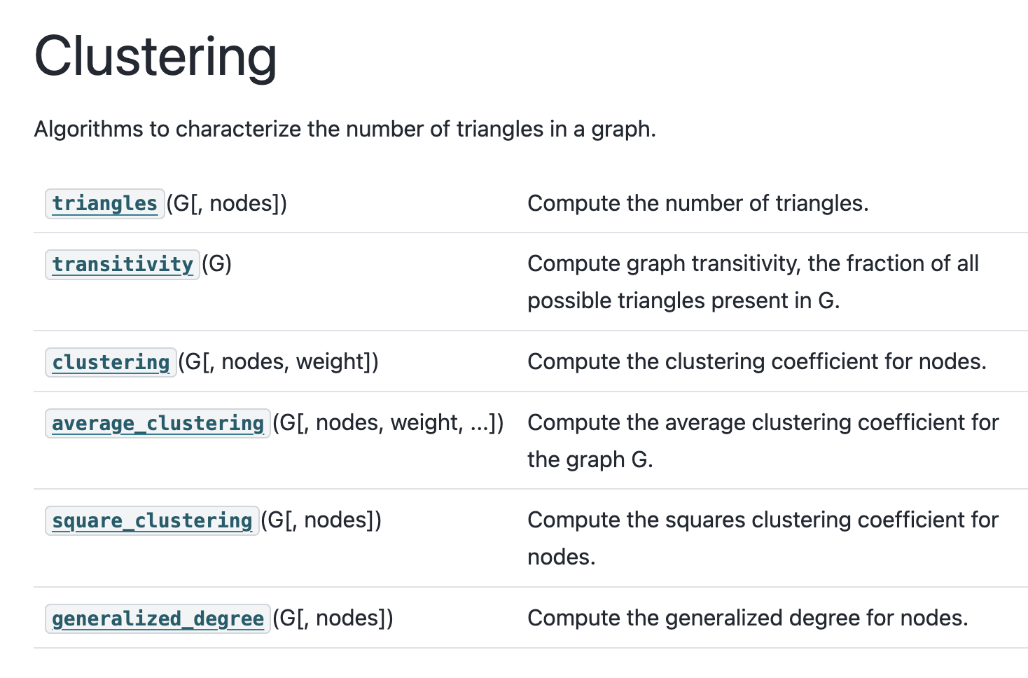
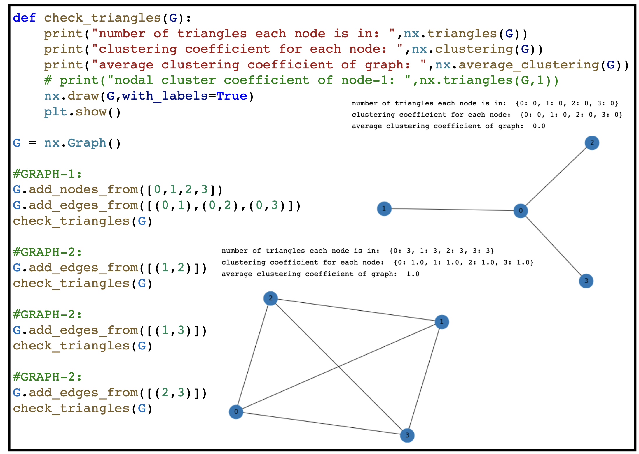
Recall: Clustering coefficient
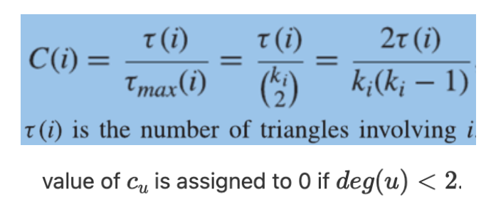
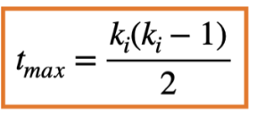
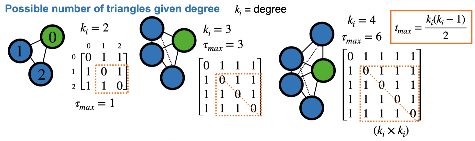
Clustering coefficient: (node property) ratio between the number of triangles that include the node, and the maximum number of triangles in which the node could participate.
Clustering coefficient \(\rightarrow\) measures triangles (friends of a friend)
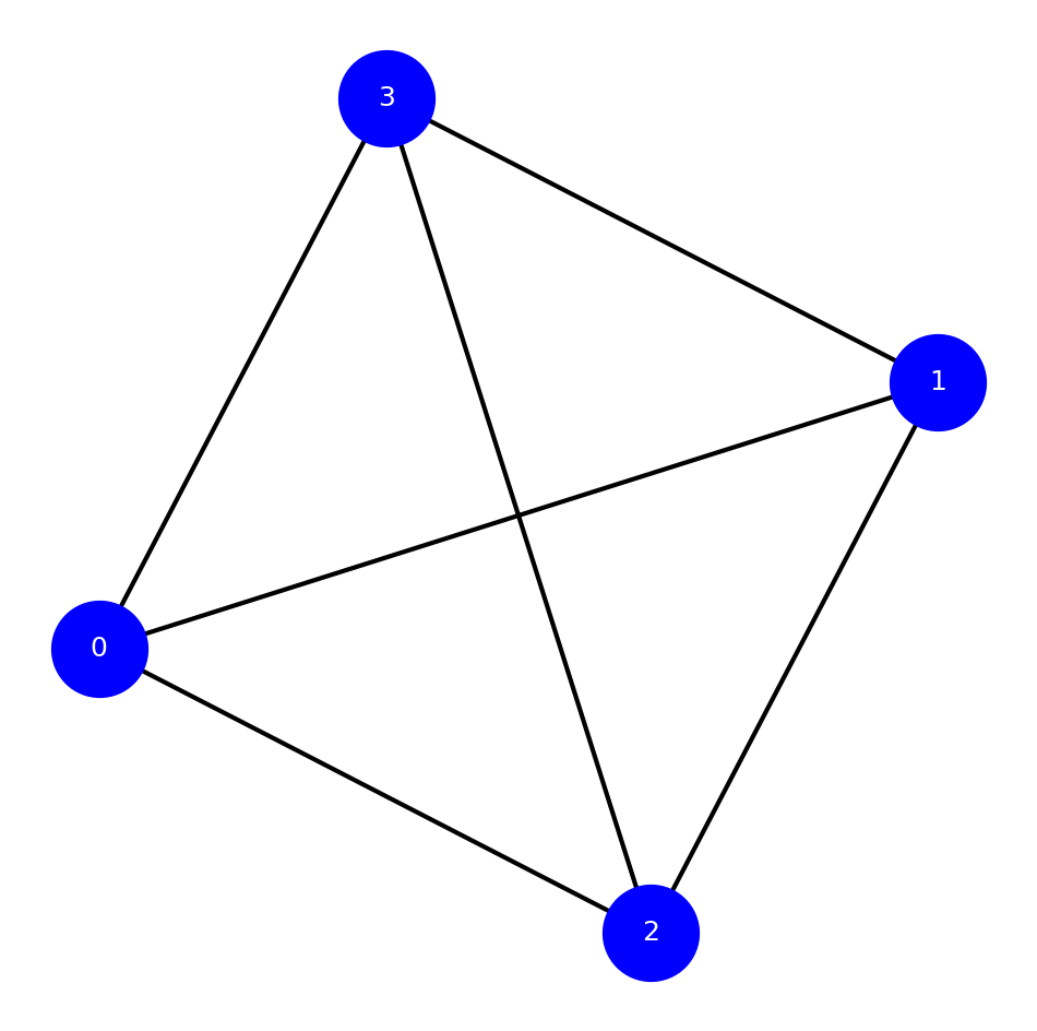
import networkx as nximport matplotlib.pyplot as pltG = nx.Graph()G.add_edges_from([(0,3),(0,2),(0,1),(1,2),(1,3),(2,3)])fig, ax = plt.subplots()fig.set_size_inches(12, 12)nx.draw(G, with_labels=True,# labels=labels, node_color='blue', width=3, node_size=4000, font_color='white', font_size=18, ax=ax )plt.show()print("number of triangles each node is in:",nx.triangles(G))print("clustering coefficient for each node:",nx.clustering(G))print("average clustering coefficient of graph:",nx.average_clustering(G))
number of triangles each node is in: {0: 3, 3: 3, 2: 3, 1: 3}
clustering coefficient for each node: {0: 1.0, 3: 1.0, 2: 1.0, 1: 1.0}
average clustering coefficient of graph: 1.0
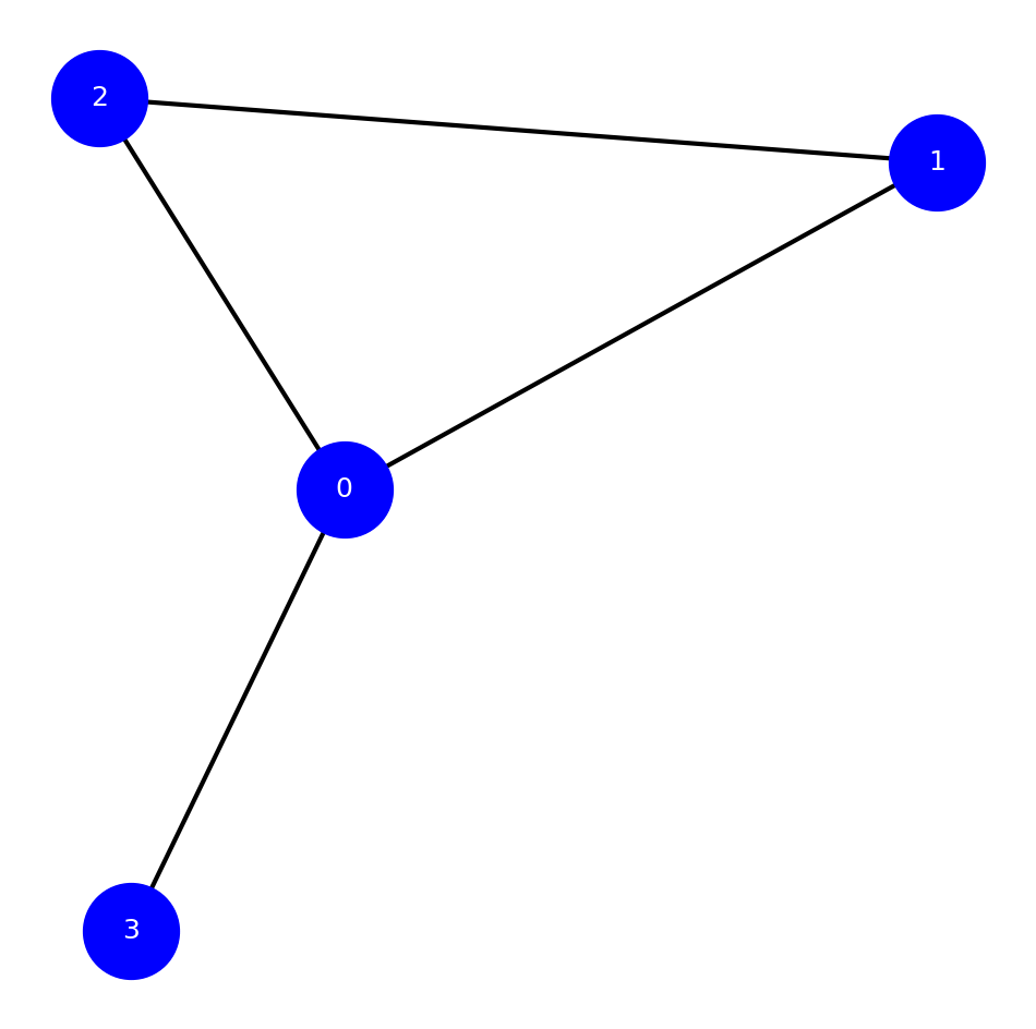
Example-2: NetworkX calculation
import networkx as nximport matplotlib.pyplot as pltG = nx.Graph()G.add_edges_from([(0,3),(0,2),(0,1),(1,2)])fig, ax = plt.subplots()fig.set_size_inches(12, 12)nx.draw(G, with_labels=True,# labels=labels, node_color='blue', width=3, node_size=4000, font_color='white', font_size=18, ax=ax )plt.show()print("number of triangles each node is in:",nx.triangles(G))print("clustering coefficient for each node:",nx.clustering(G))print("average clustering coefficient of graph:",nx.average_clustering(G))print("(0.33333333+1+1+0)/4.0=",(0.33333333+1+1+0)/4.0)
number of triangles each node is in: {0: 1, 3: 0, 2: 1, 1: 1}
clustering coefficient for each node: {0: 0.3333333333333333, 3: 0, 2: 1.0, 1: 1.0}
average clustering coefficient of graph: 0.5833333333333333
(0.33333333+1+1+0)/4.0= 0.5833333325
Additional code
Common real-world properties of networks
short paths\(\rightarrow\) it takes a few steps to go from any node to any other node.
Many triangles\(\rightarrow\) reflected in high clustering coefficients
Heterogeneous, often power law distributions, of node and link attributes (e.g. degree and weight)
Sparse\(\rightarrow\) very small average degree compared to the total number of nodes, and very small density.
Where do such properties come from?\(\rightarrow\) network modeling provides some explanatory value
Common network models
Consider building a network by adding links between a set of N disconnected nodes.
There are many ways to place the links between the nodes.
Different network models use different methods
Random Networks
Small Worlds
Configuration Model
Preferential Attachment
Other Preferential Models
Recall: Scale free (heterogenious) networks
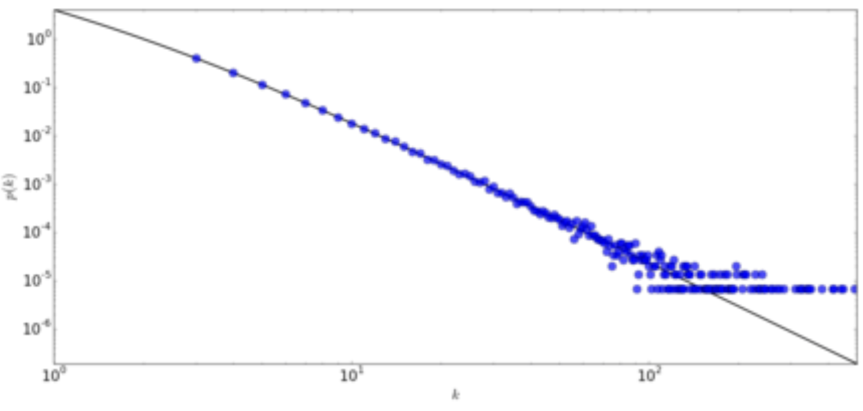
A scale-free network is a network whose degree distribution follows a power law, at least asymptotically.
That is, the fraction \(P(k)\) of nodes in the network having \(k\) connections to other nodes goes for large values of \(k\) as
\[
P(k) \sim k^{-\gamma}
\]
where \(\gamma\) is a parameter whose value is typically in the range \(2<\gamma<3\)
Degree distribution for a network with 150000 vertices and mean degree \(=6\) created using the Barabási-Albert
Scale free networks: Video
Random network model
Overview
Definition: A random network model is a mathematical abstraction used to study complex networks characterized by random connections between nodes.
Randomness: Connections between nodes are typically established randomly, following a probability distribution.
Properties:
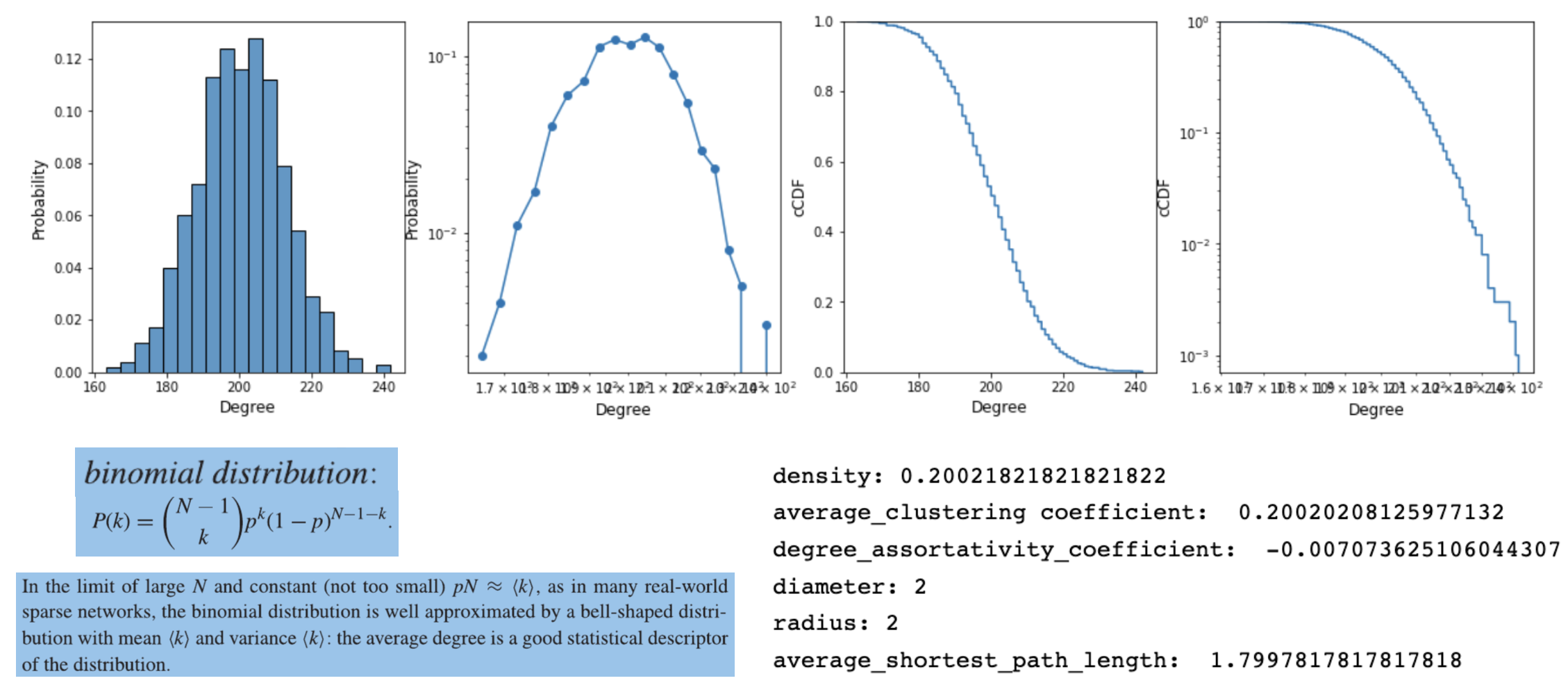
Degree Distribution: Often follows a Poisson or Gaussian distribution.
Clustering: Typically low compared to real-world networks.
Shortest Path Length: Typically shorter due to high connectivity.
Random network “recipe”
Two parameter model: The number of nodes \(N\) and a link probability \(p\) (also known as wiring probability).
The network can be constructed via the following procedure (formulated by Gilbert):
Select a pair of nodes, say \(i\) and \(j\).
Generate a random number \(r\) between 0 and 1. If \(r<p\), then add a link between \(i\) and \(j\).
Repeat (1) and (2) for all pairs of nodes.
A network built in this fashion is called a random or Erdos—Rényi network
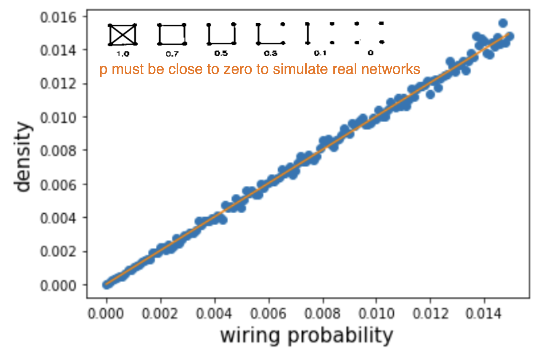
Density
Recall: Real networks are usually sparse (very small density)
Therefore, \(p\) must be close to zero to simulate real networks
Simulation: Vary wiring probability
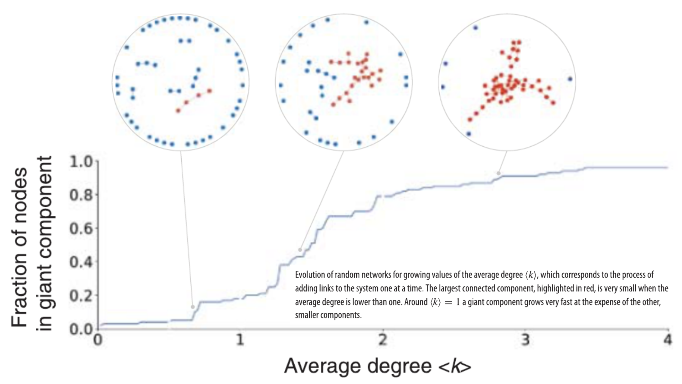
A giant component forms when (k) = 1, that is, when each node has one neighbor on average.
Evolution of random networks for growing values of the average degree \(\langle k\rangle\)
process of adding links to the system one at a time.
The largest connected component (red(), is very small when the average degree is lower than one.
Around \(\langle k\rangle=1\) a giant component grows very fast at the expense of the other, smaller components.
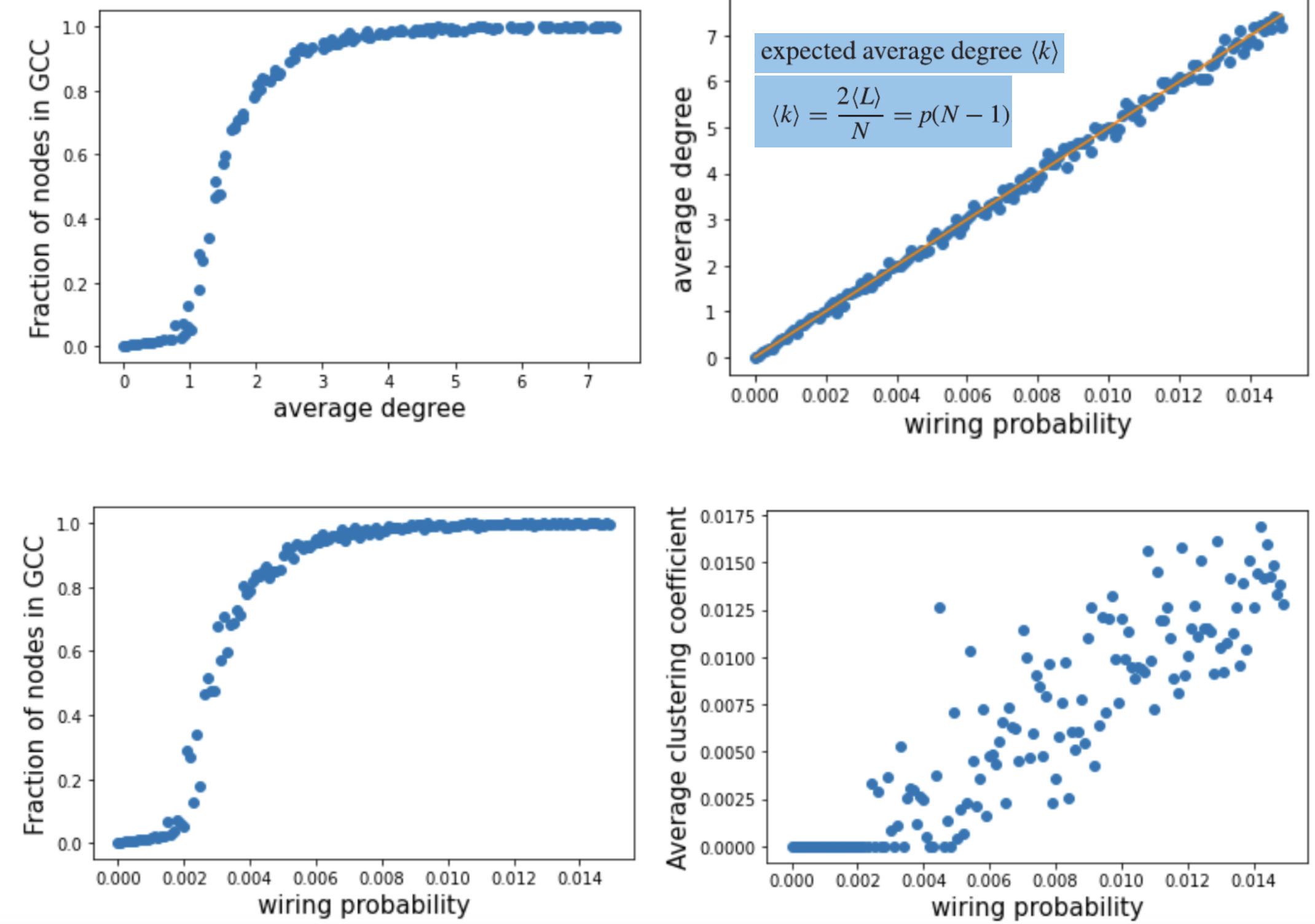
Simulation: Vary wiring probability
Vary wiring probability: N_nodes=500
NetworkX graph generator
NetworkX has functions to generate random graphs according to the Erdés—Rényi and Gilbert models:
G = nx.gnp_random_graph(N,p) # Gilbert random graph in NetworkX
Degree distribution results
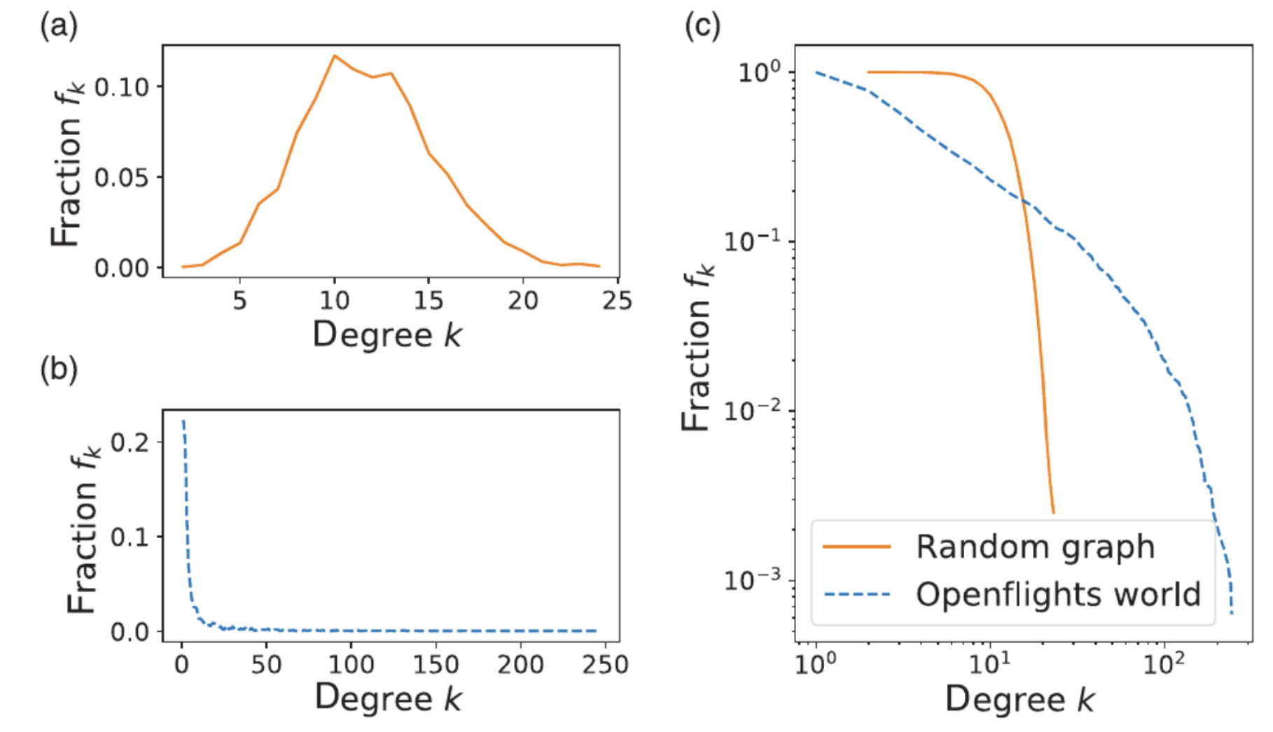
Recall: The degree-distribution of many real networks is much different from such a bell shaped distributions, due to the presence of hubs (i.e. nodes with much larger degree than the average)
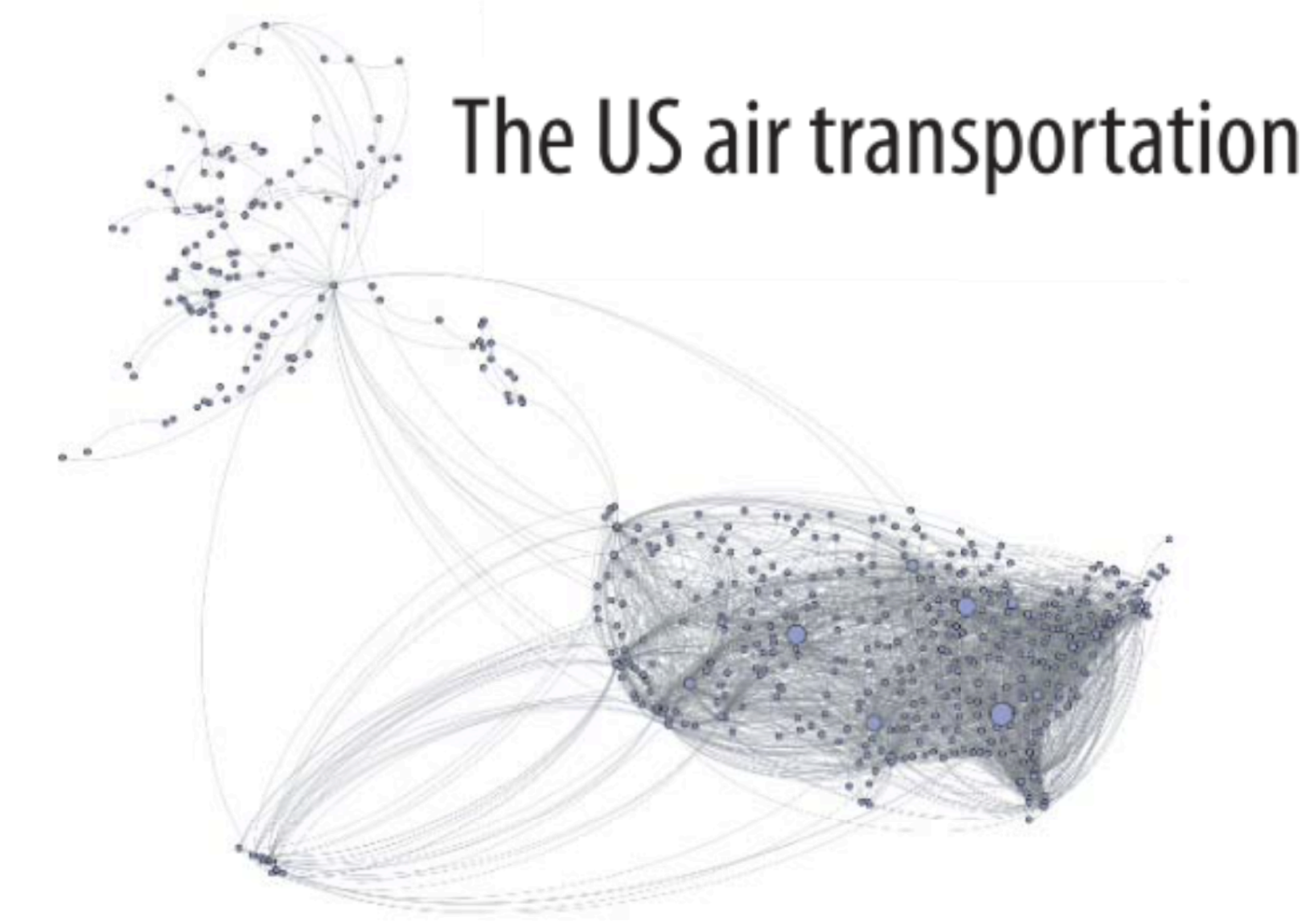
Aside: Recall World flight network
Consider the following example of a real world network
Comparison with real network
Probability distribution of degree in a random network.
Erdös-Rényi random graph with \(N=3179, L=18,617\).
Degree distribution for the world flight network: \(N=3179, L=18,617\).
Comparison between the two distributions in (a) and (b) on a double-logarithmic scale.
Pro's: Random networks do have short paths,
Cons
Triangles are rare: average clustering coefficient values can be orders of magnitude smaller than real networks
Absence of hubs \(\rightarrow\) non heterogenous degree distribution
Small World Models
Overview
In the late 1990s, Duncan J. Watts and Steven H. Strogatz introduced the small- world model, also known as the Watts—Strogatz model.
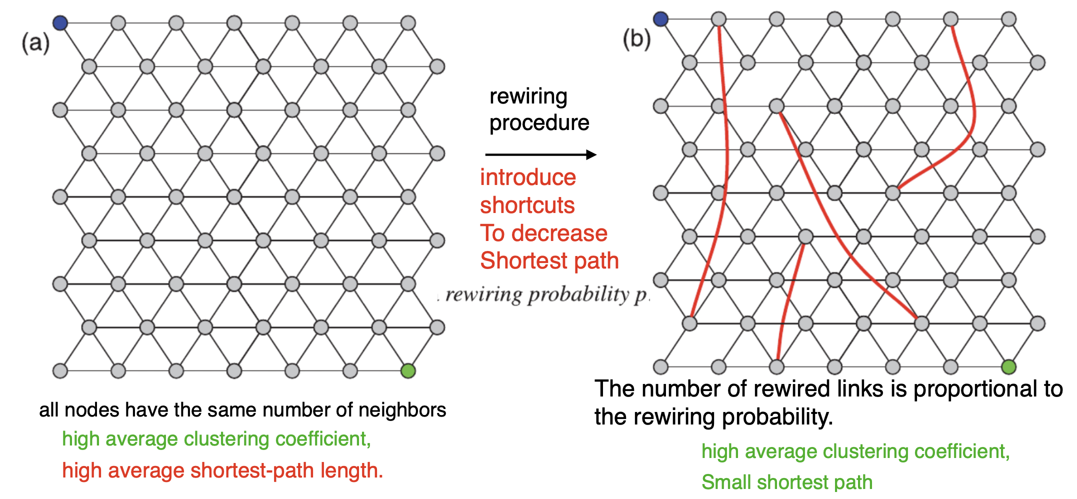
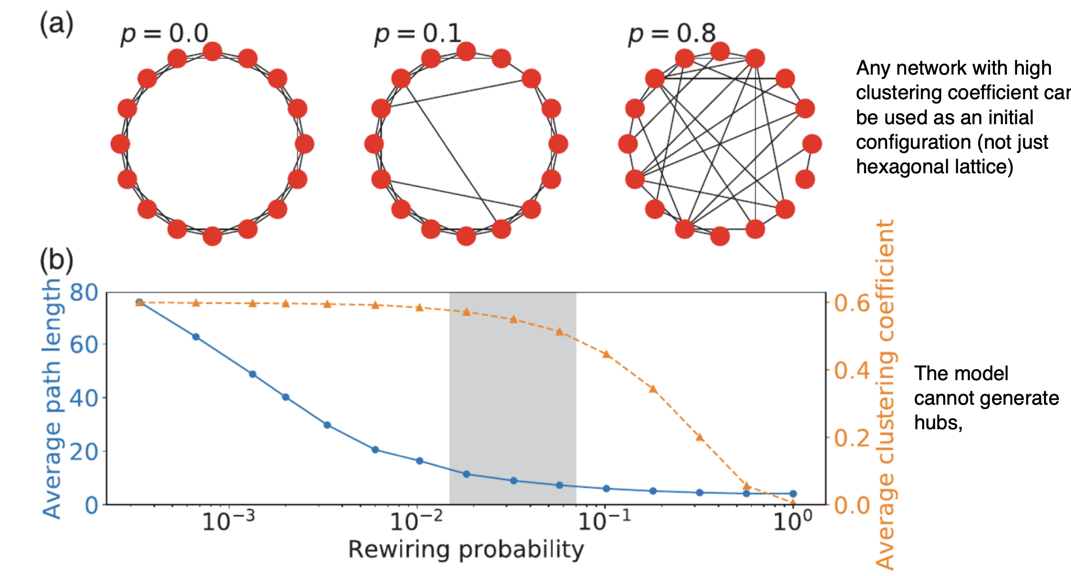
Goal: Create a model with short paths and high clustering coefficient.
Definition: A small-world network model is characterized by a combination of high clustering (local inter-connectivity) and short average path lengths between nodes.
Key Features:
High Clustering: Nodes tend to cluster together, forming tightly knit groups.
Short Average Path Lengths: Despite clustering, the average number of steps required to connect any two nodes is relatively small.
Randomness and Regularity: Combines elements of regular and random networks.
Properties:
Clustering Coefficient: High compared to random networks.
Average Path Length: Short, comparable to random networks.
Small World Phenomenon: Nodes are only a few steps away from each other despite clustering.
Recipe
The algorithm for generating a small-world network is as such:
Begin with a ring of \(N\) nodes
Connect each node to its \(k\) nearest neighbors (or \(k-1\) if \(\mathrm{k}\) is odd).
For each edge \((u, v)\), with probability \(p\), replace edge \((u, v)\) with \((u, w)\) where \(w\) is not a neighbor of \(u\).
The expected number of rewired links is \(p L\), where \(p\) is the rewiring probability and \(L\) is the total number of links in the network. The special case \(p=0\) corresponds to the initial lattice, and the special case \(p=1\) yields a random network.
NetworkX
varying model parameters
If p is chosen to be neither too small nor too large, it is possible to achieve a trade-off, where there are enough shortcuts to make the distances considerably smaller on average, but not so many as to disrupt most of the triangles
In this regime, the paths are as short as those in random networks, while the average clustering coefficient decreases only slightly with respect to the initial lattice configuration, so that it can be comparable with that of real social networks.
Configuration Models
Overview
Goal: Given some degree distribution, can we construct a network whose nodes have exactly that degree distribution?
Setup
Consider an arbitrary degree sequence, with node 1 having degree k1, node 2 degree k2, … etc
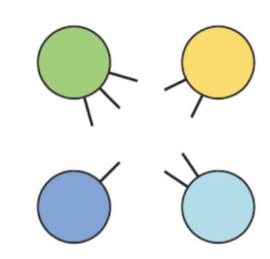
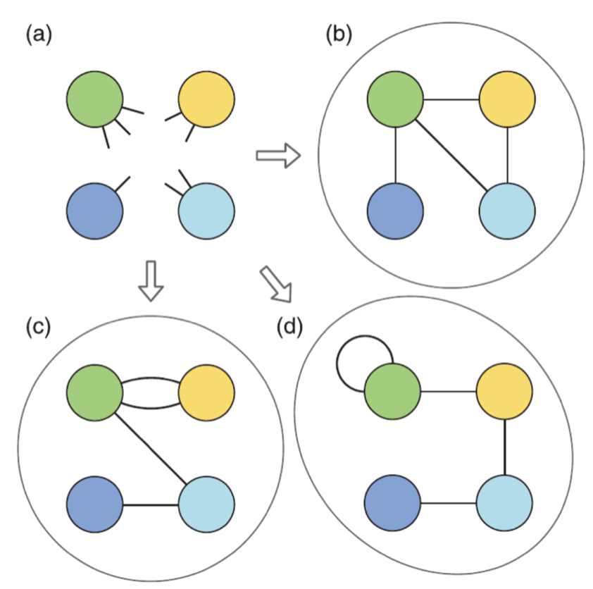
The first step is to assign to each node a number of stubs corresponding to the degree of the node
Form links:
A pair of stubs is selected at random and joined to each other
This forms a link between the nodes attached to the stubs.
Repeat until all stubs are joined in pairs.
Pros and Cons
Pros:
Can make networks with correct degree distribution
Easy to use in NetworkX\(\rightarrow\)G = nx.configuration_model(D) # network with degree sequence D
Cons:
Lacks explanatory power
Requires an a-priori degree sequence
The Generated networks aren’t unique (multiple ways to create the same network)
Only reproduces correct degree distribution but not necessarily other desired properties
Preferential Attachment Models
Motivation
The models explored so far are static (number of nodes was constant)
Real networks, instead, are usually dynamic. Nodes and links appear and disappear.
The models explored so far cannot explain the existence of hubs.
i.e. linking rules are basically egalitarian - the nodes choose their neighbors totally at random.
in this case, unlikely for any one node to have an advantage over the other nodes or end up with more neighbors than the rest (unrealistic).
Overview
Definition: Preferential Attachment is a network growth model where new nodes preferentially attach to existing nodes with higher degrees.
Key Principle: Nodes that already have more connections (higher degree nodes) are more likely to attract new connections.
Mathematical Formulation: Probability of a new node connecting to an existing node ( i ) is proportional to the degree ( k_i ) of node ( i ).
Resulting Network Properties:
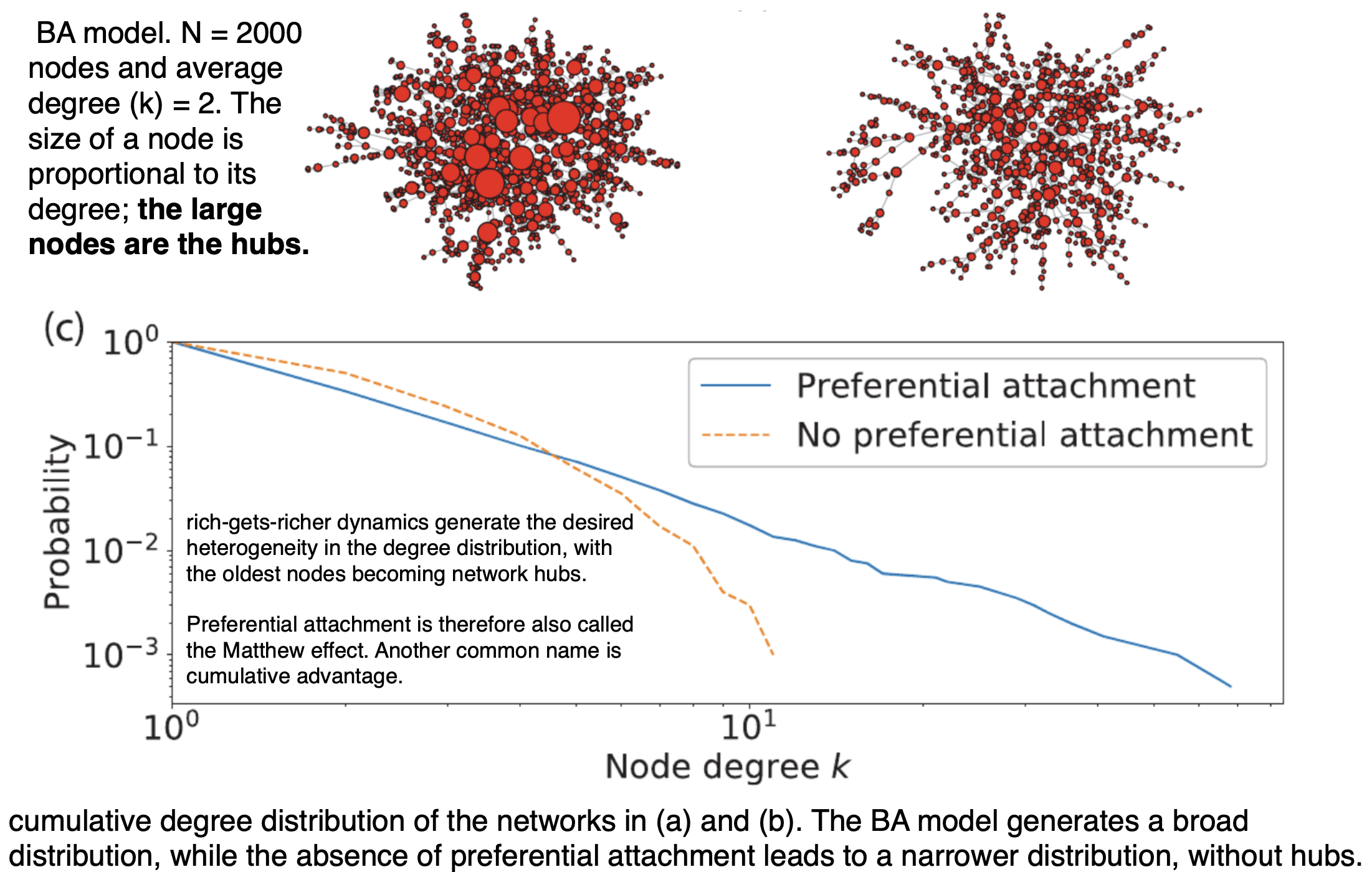
Power Law Degree Distribution: Leads to a distribution where a few nodes have many connections (hubs) and many nodes have few connections.
Rich-get-Richer Effect: Nodes with higher degrees tend to accumulate more connections over time.
Applications: Used to model various real-world networks like social networks, citation networks, and the World Wide Web.
Criticism and Enhancements: Criticized for oversimplifying real-world dynamics; enhanced models may incorporate additional factors like node fitness or geographical constraints.
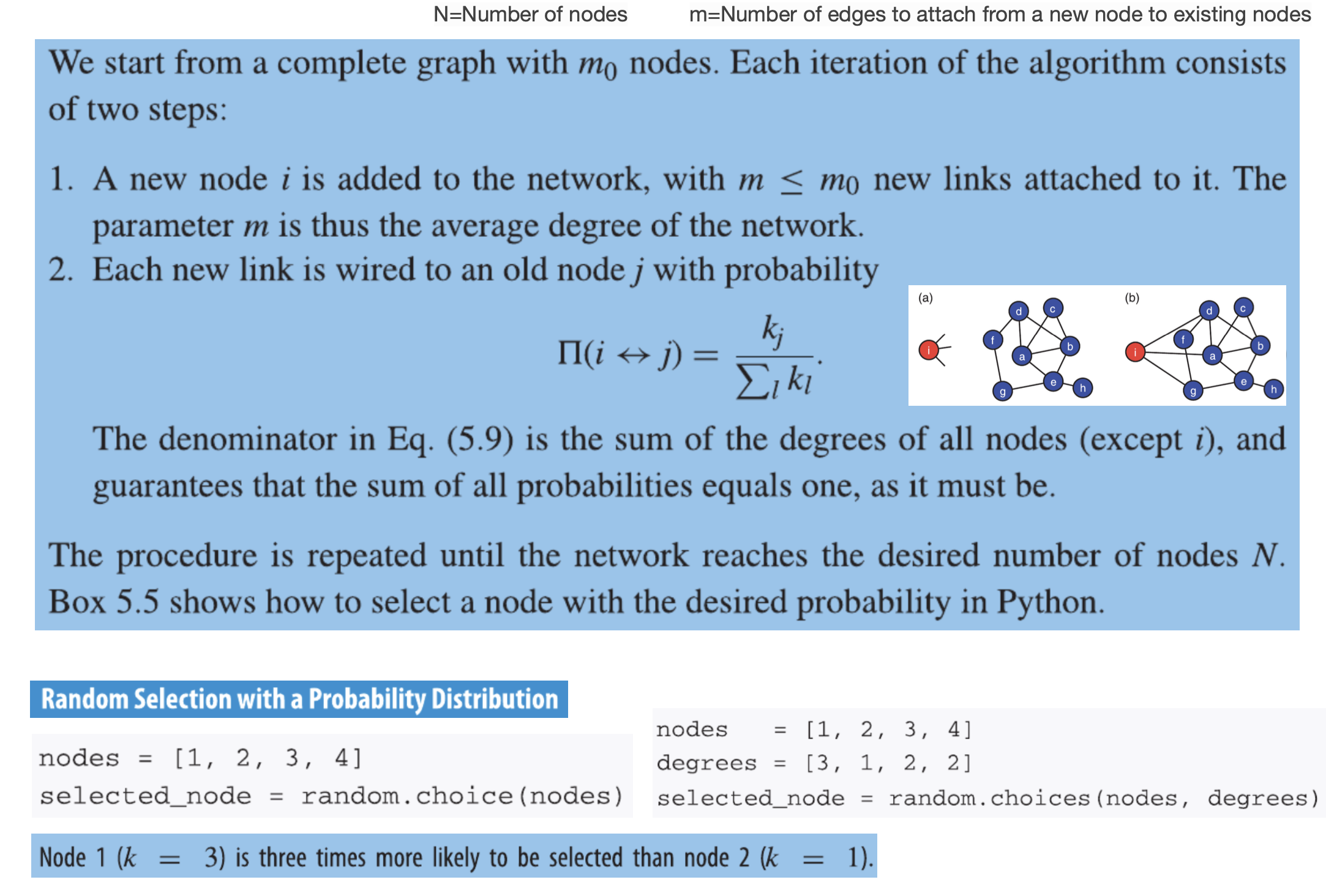
Growth mechanism
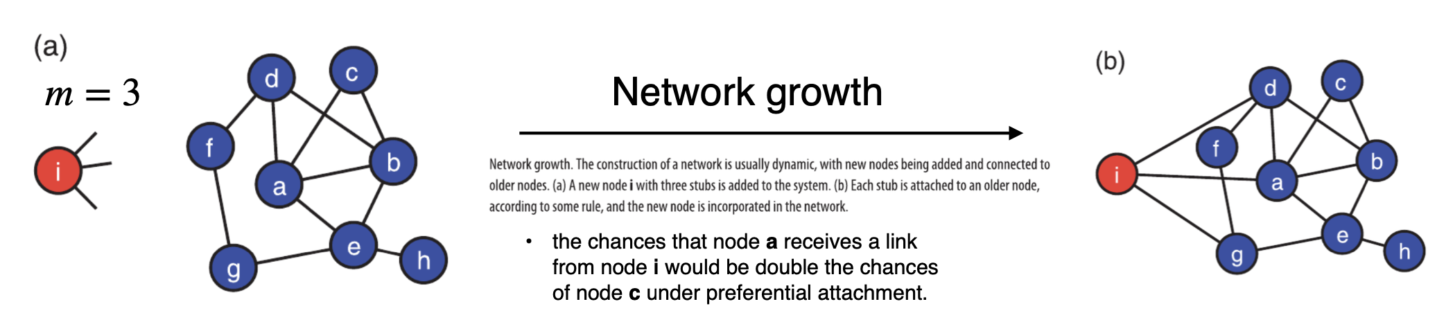
Preferential attachment: high-degree nodes have a high probability of receiving new links
The probability that a new node is attached to an old node is proportional to the degree of the old node.
The best-known network growth model incorporating preferential attachment Barabdsi-Albert model (1999) (AKA BA model or preferential attachment model)
At each step, a new node is added and connected to some existing nodes.
a node with degree 100 is 100 times more likely to receive a new link than a node with degree one.
Algorithm
G=nx.barabasi_albert_graph(N,m) \# BA model network
Example
Network generated via a similar growth model, but with random rather than preferential attachment –> no hubs.
Limitations of BA model
Dependency on linear preferential attachment,
It yields a fixed pattern for the degree distribution: The slope of the preferential attachment curve is the same for any choice of the model parameters.
Real degree distributions could decay faster or more slowly.
The hubs are the oldest nodes; new nodes cannot overcome them in degree.
It does not create many triangles. The average clustering coefficient is much lower than in many real networks.
Nodes and links are only added; in real networks they can also be deleted.
Since each node is attached to older nodes, the network consists of a single connected component. Many real networks have multiple components.
Doesn’t work with singletons, Its degree is zero, so the probability that it will get links is also zero: the node will never have neighbors!
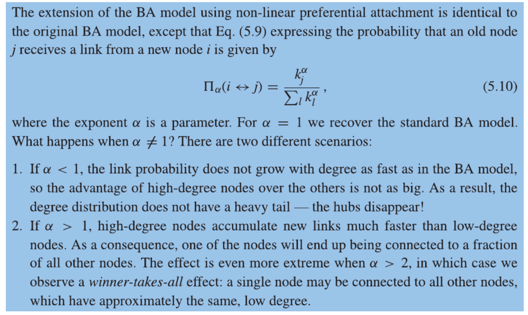
Modification-1: Non-linear attachment
BA model uses linear preferential attachment, in that the link probability is strictly proportional to the degree of the target node.
This exposes a fundamental fragility of the BA model, as the necessity of strict proportionality between link probability and degree appears unrealistic.
probability vary as some power of the degree. (non-linear preferential attachment)
Modification-2: Attractiveness Model
A node receives links because of its degree, AND also because it has an intrinsic attractiveness.
In the attractiveness model, the link probability is proportional to the sum of degree and a “attractiveness” constant.
The attractiveness model is a slightly modified version of the original BA model, in which Eq. (5.9) expressing the probability that an old node \(j\) receives a link from a new node \(i\) is replaced by \[
\Pi(i \leftrightarrow j)=\frac{A+k_j}{\sum_l\left(A+k_l\right)},
\]
where \(A\) is the attractiveness parameter and can take any positive value. The case \(A=0\) yields the BA model.
For any value of the attractiveness parameter \(\mathrm{A}\), the model builds networks with heavy- tailed degree distributions.
The slope of the distribution depends on A.This way, the model is able to match degree distributions of multiple real networks, unlike the BA model.
Modification-3: Fitness Model
In BA and attractiveness model the hubs are also the oldest nodes.
Not always true (new players come along and shake things up)
Fitness model in which each node has its own individual appeal, called fitness.
The fitness values are intrinsic features of the nodes; they do not change over time.
The link probability is proportional to the product of the degree and the fitness of the target node. The fitness model is similar to the BA model, but each node \(i\) is assigned a fitness value \(\eta_i>0\) generated from some distribution \(\rho(\eta)\). Then at every step, each new link from a new node \(i\) is wired to an old node \(j\) with probability \[
\Pi(i \leftrightarrow j)=\frac{\eta_j k_j}{\sum_l \eta_l k_l} .
\]
If all nodes have identical fitness, the model reduces to the BA model, as the constant \(\eta\) is a factor that cancels out between numerator and denominator of Eq. (5.12), returning the standard prescription of preferential attachment.
If the fitness distribution \(\rho(\eta)\) has infinite support (i.e. \(\eta\) can take arbitrarily large values), then there is a winner-takes-all effect with the highest-fitness node being linked to most modes. But if the fitness distribution \(\rho(\eta)\) has finite support (i.e. \(\eta\) has a finite maximum value), then the degree distribution of the model has a heavy tail. An example of this case is the uniform distribution in the unit interval. In Python we can draw fitness values with uniform distribution using the random() function.
Modification-4: Triadic closure
Networks built with the BA model have very low clustering coefficients (i.e. they don’t have many triangles), which often isn’t realistic
This is because the model has no built in mechanism for triangle generation
In the BA model the probability of a node receiving a link is proportional to its degree, regardless of whether the new pair of neighbors have a common edge or not.
BA only weights pair-wise connections, three body connections (neighbors of neighbors) are not considered
The formation of a triangle via the addition of a link is called triadic closure. This is a very important link-formation mechanism in social networks
Rank model: Overview
Preferential attachment implies that the nodes have a perception of how important other nodes are (i.e. new nodes “know” the degree of the target nodes)
In realistic settings, it is more common to have a perception of the relative value of things, rather than of their absolute value.
I.e. it is easier to rank than to guess the value. For example, you may know someone is older than you without knowing their exact age.
General idea: - rank nodes based some properties, e.g. degree. \(\rightarrow\) Rank vector: \(R=(1,2,3,4)\) - nodes receive new links with probability proportional to some inverse power of their rank with exponential parameter \(\alpha\). \(\mathrm{R}=(1,2,3,4) \rightarrow \mathrm{p} \approx(0.1,0.05,0.033,0.025)\) (if \(\alpha=1)\)
Rank model: Algorithm
The rank model can start from any small graph with \(m_0\) nodes. A node property, such as the degree, age, or some measure of fitness is selected to rank the nodes.
Each iteration of the algorithm consists of the following steps:
All nodes are ranked based on the property of interest. Nodes are assigned ranks \(R=1,2\), etc. Node \(l\) receives rank \(R_l\).
A new node \(i\) is added to the network, with \(m \leq m_0\) new links attached to it.
Each new link from \(i\) is wired to an old node \(j\) with probability
Nodes may have to be re-ranked at each iteration if the ranking property depends on the links from new nodes joining the network, as happens for example when nodes are ranked by degree.
rank model generates networks with heavy-tailed degree distributions,
By tuning the exponent, it is possible to vary the shape of the distribution, and to reproduce the empirical distributions observed in many real-world networks.
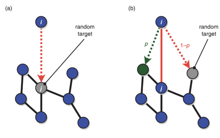
Random walk model
The random walk model can start from any small network. Each iteration of the algorithm consists of the following steps:
A new node \(i\) is added to the network, with \(m>1\) new links attached to it.
The first link is wired to an old node \(j\), chosen at random.
Each other link is attached to a randomly selected neighbor of \(j\), with probability \(p\), or to another randomly selected node, with probability \(1-p\).
The parameter \(p\) is the probability of triadic closure, because by setting a link between \(i\) and a neighbor of \(j\), say \(l\), we close the triangle \((i, j, l)\). If \(p=0\), there is no triadic closure and new nodes choose their neighbors entirely at random. When \(p=1\) all links except the first one are wired to neighbors of the initially selected old node, thus closing triangles.
Random walk model: Important features
New nodes “explore” the system randomly. They have NO knowledge of the degrees of old nodes (which is more realistic than BA).
Nodes are “discovered” with a frequency proportional to their degrees. Therefore, the process of triadic closure implicitly induces preferential attachment.
The strict proportionality between link probability and degree, needed to generate broad degree distributions, can be enforced by simple random mechanisms
Finally, when \(p\) is large enough that there is a sufficiently high density of triangles, the random walk model produces networks with community structures
Summary
Concluding summary
These summaries capture the essence of each model’s mechanisms and their contributions to understanding network structure and dynamics.
Erdős-Rényi Model:
All nodes have equal probability of connection.
Short paths but lacks triangles and hubs.
Small-World Model:
Adds random shortcuts to a lattice structure.
Maintains high clustering with reduced path lengths.
Unable to create hubs effectively.
Configuration Model:
Generates networks with specified degree sequences.
Used as a baseline to study effects beyond degree distribution.
Network Growth Models:
Nodes and links added over time.
Matches real-world network evolution like the Internet.
Preferential Attachment:
Higher degree nodes attract more connections (hubs).
Key mechanism explaining hub emergence.
Barabási-Albert Model:
Combines growth and preferential attachment.
Generates networks with heavy-tailed degree distributions (hubs).
Implicit Preferential Attachment:
Seen in processes like triadic closure and link selection.
Enhancements to Barabási-Albert Model:
Introduces attractiveness, fitness, triadic closure, and ranking.
Overcomes limitations to better simulate real-world networks.