## simple matrix inversion
import numpy as np

A = np.array([[4, 7], [2, 6]])

print(np.linalg.inv(A))
[[ 0.6 -0.7]
[-0.2 0.4]]A quick math review
3Blue1Brown, Essence of Linear Algebra: A staple resource for building geometric intuition, covering vectors, span and basis, linear transformations, determinants, column and null space, dot products, change of basis, and eigenvectors and eigenvalues. The playlist is roughly 16 short videos that give you a strong visual grasp of what each operation actually does.
The following is an embedded Playlist, once the first video ends, the following video should start automatically. You can also access the full playlist at the link below the video.
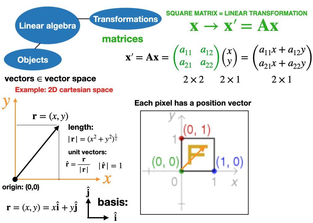
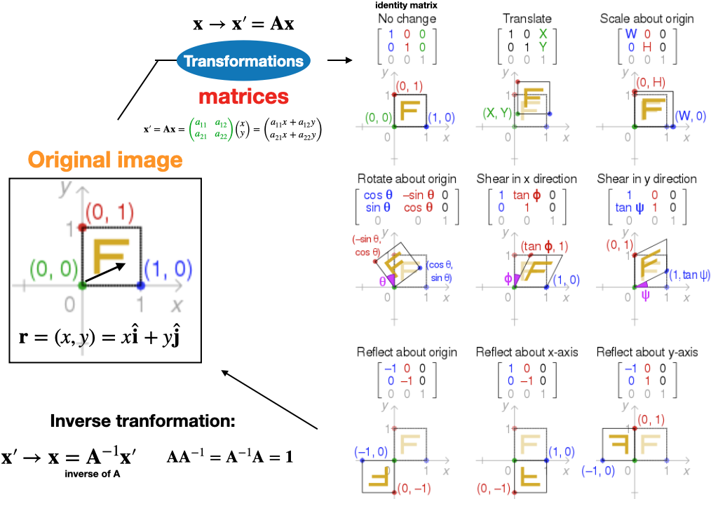
Key insight the columns of \(A\) are exactly where the standard basis vectors \(\mathbf{e}_1, \mathbf{e}_2\) land after transformation.
\[A = \begin{pmatrix} a & b \\ c & d \end{pmatrix}, \quad \mathbf{e}_1 = \begin{pmatrix} 1 \\ 0 \end{pmatrix}, \quad \mathbf{e}_2 = \begin{pmatrix} 0 \\ 1 \end{pmatrix}\]
\[A\mathbf{e}_1 = \begin{pmatrix} a & b \\ c & d \end{pmatrix}\begin{pmatrix} 1 \\ 0 \end{pmatrix} = \begin{pmatrix} a \\ c \end{pmatrix} \leftarrow \text{column 1}\]
\[A\mathbf{e}_2 = \begin{pmatrix} a & b \\ c & d \end{pmatrix}\begin{pmatrix} 0 \\ 1 \end{pmatrix} = \begin{pmatrix} b \\ d \end{pmatrix} \leftarrow \text{column 2}\]
Example: a 90° counter-clockwise rotation
\[A = \begin{pmatrix} 0 & -1 \\ 1 & 0 \end{pmatrix} \quad \rightarrow \quad \mathbf{e}_1 = \begin{pmatrix} 1 \\ 0 \end{pmatrix} \mapsto \begin{pmatrix} 0 \\ 1 \end{pmatrix}, \quad \mathbf{e}_2 = \begin{pmatrix} 0 \\ 1 \end{pmatrix} \mapsto \begin{pmatrix} -1 \\ 0 \end{pmatrix}\]
Why this matters: Any vector \(\mathbf{x} = x_1\mathbf{e}_1 + x_2\mathbf{e}_2\) transforms linearly, so its image under \(A\) is
\[ \tilde{\mathbf{x}} = A\mathbf{x} = x_1 A\mathbf{e}_1 + x_2 A\mathbf{e}_2=x_1\tilde{\mathbf{e}}_1+x_2\tilde{\mathbf{e}}_2, \]
where \(\tilde{\mathbf{x}}\) denotes the transformed vector. Because \(A\mathbf{e}_1\) and \(A\mathbf{e}_2\) are just the images of the basis vectors (the columns of \(A\)), knowing where each basis vector goes (i.e., \(\mathbf{e}_1 \mapsto \tilde{\mathbf{e}}_1 = A\mathbf{e}_1\), \(\mathbf{e}_2 \mapsto \tilde{\mathbf{e}}_2 = A\mathbf{e}_2\)) tells you everything about how \(A\) transforms all vectors.
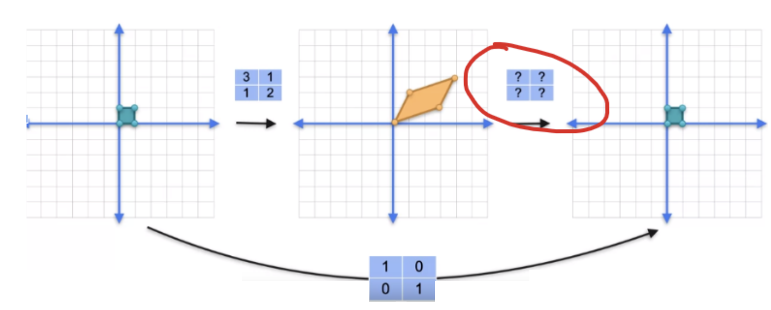
A square matrix \(A\) is invertible if there exists a matrix \(A^{-1}\) such that:
\[ A A^{-1}=A^{-1} A=I \]
(where \(I\) is the identity matrix). A matrix has an inverse if and only if its determinant is non-zero ( \(\operatorname{det}(A) \neq 0\) ).
## simple matrix inversion
import numpy as np
A = np.array([[4, 7], [2, 6]])
print(np.linalg.inv(A))[[ 0.6 -0.7]
[-0.2 0.4]]Simple \(2 \times 2\) Example To find the inverse of a \(2 \times 2\) matrix, swap the positions of \(a\) and \(d\), put negative signs in front of \(b\) and \(c\), and divide everything by the determinant \((a d-b c)\).
Matrix \(A\) :
\[ A=\left(\begin{array}{ll} 4 & 7 \\ 2 & 6 \end{array}\right) \]
1 Find Determinant: \(\operatorname{det}(A)=(4 \times 6)-(7 \times 2)=24-14=10\) 2 Apply \(2 \times 2\) Formula:
\[ A^{-1}=\frac{1}{10}\left(\begin{array}{cc} 6 & -7 \\ -2 & 4 \end{array}\right)=\left(\begin{array}{cc} 0.6 & -0.7 \\ -0.2 & 0.4 \end{array}\right) \]
x=np.array([[1, 0, 2], [2, -1, 3], [4, 1, 8]])
print(np.linalg.inv(x))
[[-11. 2. 2.]
[ -4. -0. 1.]
[ 6. -1. -1.]]Find the inverse (\(A^{-1}\)) of the following matrix \(A\):
\[A = \begin{pmatrix} 1 & 0 & 2 \\ 2 & -1 & 3 \\ 4 & 1 & 8 \end{pmatrix}\]
We will expand along the first row because it contains a zero, which makes the math easier.
\[\det(A) = 1 \cdot \begin{vmatrix} -1 & 3 \\ 1 & 8 \end{vmatrix} - 0 \cdot \begin{vmatrix} 2 & 3 \\ 4 & 8 \end{vmatrix} + 2 \cdot \begin{vmatrix} 2 & -1 \\ 4 & 1 \end{vmatrix}\]
\[\det(A) = 1(-11) - 0 + 2(6) = -11 + 12 = 1\]
Since \(\det(A) = 1\) (which is non-zero), the matrix is invertible.
For each element, temporarily cross out its row and column, and calculate the determinant of the remaining 2x2 matrix.
Top Row:
\(M_{11} = \begin{vmatrix} -1 & 3 \\ 1 & 8 \end{vmatrix} = -11\)
\(M_{12} = \begin{vmatrix} 2 & 3 \\ 4 & 8 \end{vmatrix} = (16 - 12) = 4\)
\(M_{13} = \begin{vmatrix} 2 & -1 \\ 4 & 1 \end{vmatrix} = (2 - (-4)) = 6\)
Middle Row:
\(M_{21} = \begin{vmatrix} 0 & 2 \\ 1 & 8 \end{vmatrix} = (0 - 2) = -2\)
\(M_{22} = \begin{vmatrix} 1 & 2 \\ 4 & 8 \end{vmatrix} = (8 - 8) = 0\)
\(M_{23} = \begin{vmatrix} 1 & 0 \\ 4 & 1 \end{vmatrix} = (1 - 0) = 1\)
Bottom Row:
\(M_{31} = \begin{vmatrix} 0 & 2 \\ -1 & 3 \end{vmatrix} = (0 - (-2)) = 2\)
\(M_{32} = \begin{vmatrix} 1 & 2 \\ 2 & 3 \end{vmatrix} = (3 - 4) = -1\)
\(M_{33} = \begin{vmatrix} 1 & 0 \\ 2 & -1 \end{vmatrix} = (-1 - 0) = -1\)
Putting them together gives the Matrix of Minors:
\[\text{Minors} = \begin{pmatrix} -11 & 4 & 6 \\ -2 & 0 & 1 \\ 2 & -1 & -1 \end{pmatrix}\]
Apply a grid of alternating signs \(\begin{pmatrix} + & - & + \\ - & + & - \\ + & - & + \end{pmatrix}\) to the matrix of minors. This changes the sign of elements at \(M_{12}\), \(M_{21}\), \(M_{23}\), and \(M_{32}\):
\[\text{Cofactors}(C) = \begin{pmatrix} -11 & -4 & 6 \\ 2 & 0 & -1 \\ 2 & 1 & -1 \end{pmatrix}\]
Flip the rows and columns of the cofactor matrix (row 1 becomes column 1, etc.).
\[\text{adj}(A) = C^T = \begin{pmatrix} -11 & 2 & 2 \\ -4 & 0 & 1 \\ 6 & -1 & -1 \end{pmatrix}\]
The formula is \(A^{-1} = \frac{1}{\det(A)} \cdot \text{adj}(A)\). Since our determinant is \(1\), the adjugate matrix is our final answer!
\[A^{-1} = \frac{1}{1} \begin{pmatrix} -11 & 2 & 2 \\ -4 & 0 & 1 \\ 6 & -1 & -1 \end{pmatrix} = \begin{pmatrix} -11 & 2 & 2 \\ -4 & 0 & 1 \\ 6 & -1 & -1 \end{pmatrix}\]
(To double-check this, multiplying \(A \times A^{-1}\) will result in the 3x3 Identity Matrix).
Invertible: \(A\) is a one-to-one, reversible transformation of space
Non-Invertible (Singular): \(A\) collapses space into a lower-dimensional subspace
Simple example:
\[A = \begin{pmatrix} 2 & 0 \\ 0 & 3 \end{pmatrix} \xrightarrow{\text{invertible}} \text{stretches plane, } \det = 6\]
\[B = \begin{pmatrix} 1 & 2 \\ 2 & 4 \end{pmatrix} \xrightarrow{\text{singular}} \text{collapses plane to a line, } \det = 0\]
Key intuition: invertibility is about whether \(A\) preserves the “richness” of space, singular matrices are the ones that irreversibly flatten it.
The two columns of \(A\) are the transformed basis vectors \(\tilde{\mathbf{e}}_1= (a_{11}, a_{21})^{\top}\) and \(\tilde{\mathbf{e}}_2=(a_{12}, a_{22})^{\top}\), which form a parallelogram.
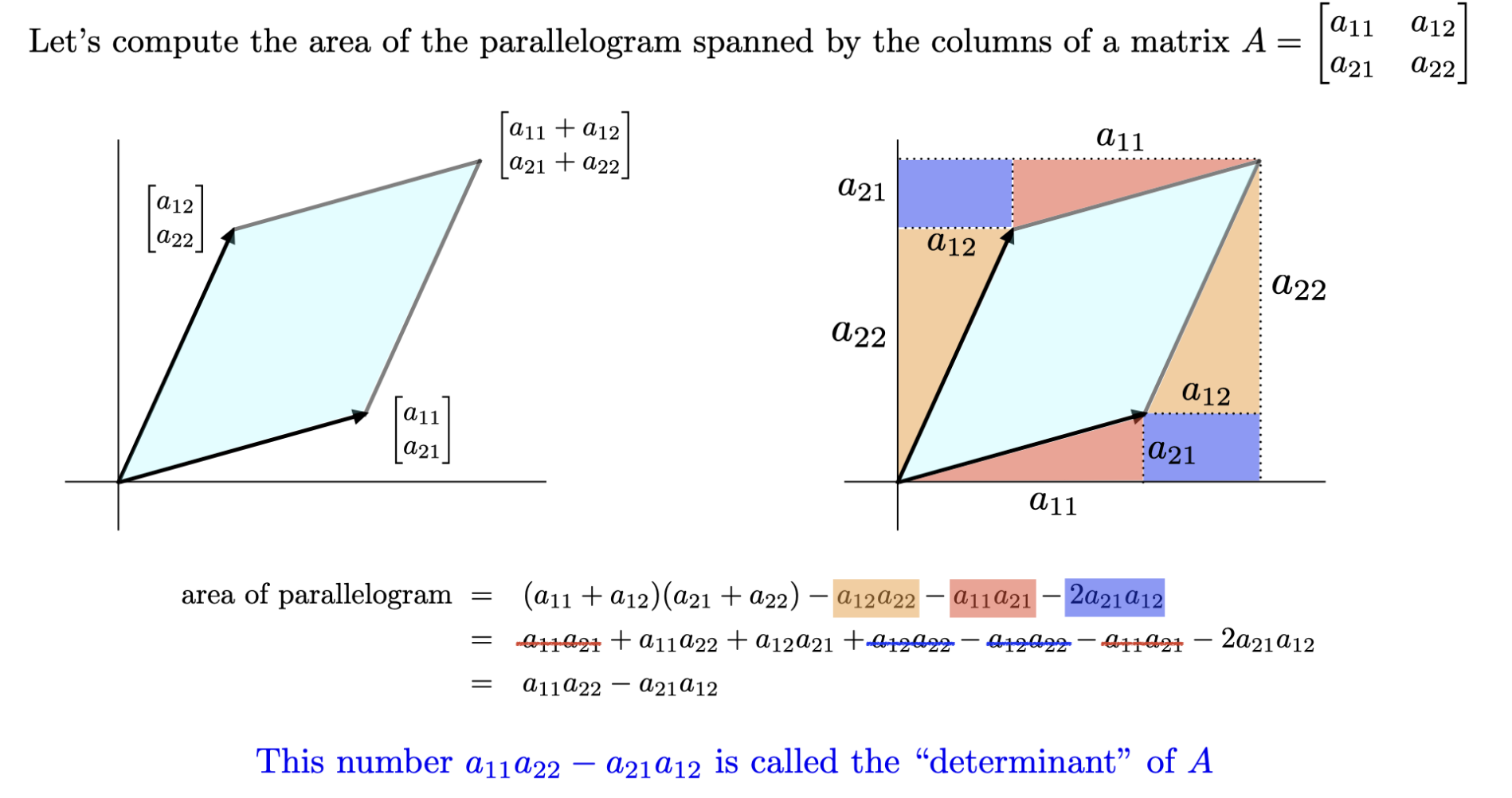
Algebraically a scalar \(\det(A)\) computed from an \(n \times n\) matrix that encodes whether \(A\) is invertible
Geometrically \(|\det(A)|\) is the factor by which \(A\) scales volume
\[\det\begin{pmatrix} a & b \\ c & d \end{pmatrix} = ad - bc\]
| \(\det(A)\) | Meaning |
|---|---|
| \(= 0\) | \(A\) collapses space: not invertible |
| \(> 0\) | Volume scaled by \(\det(A)\), orientation preserved |
| \(< 0\) | Volume scaled by \(|\det(A)|\), orientation flipped |
| \(= 1\) | Volume unchanged (e.g., rotation) |
2D example columns \(\mathbf{a}_1, \mathbf{a}_2\) form a parallelogram: \(|\det(A)|\) is its area
\[A = \begin{pmatrix} 3 & 0 \\ 0 & 2 \end{pmatrix} \rightarrow \det(A) = 6 \quad \text{(unit square} \mapsto \text{rectangle of area 6)}\]
\[B = \begin{pmatrix} 2 & 1 \\ 1 & 2 \end{pmatrix} \rightarrow \det(B) = (2)(2) - (1)(1) = 4 - 1 = 3 \quad \text{(unit square} \mapsto \text{parallelogram of area 3)}\]
Key properties
All these conditions are equivalent for an \(n \times n\) matrix \(A\)! (If any one is true, all are true; if any one is false, all are false.)
All these conditions say the same thing \(A\) loses no information.
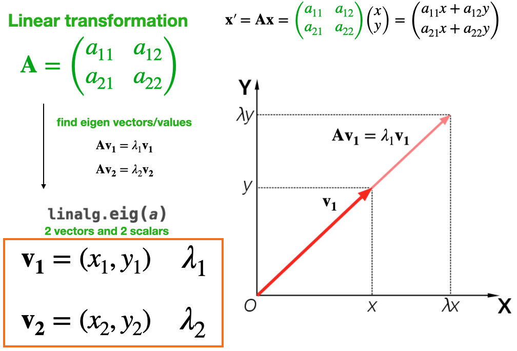
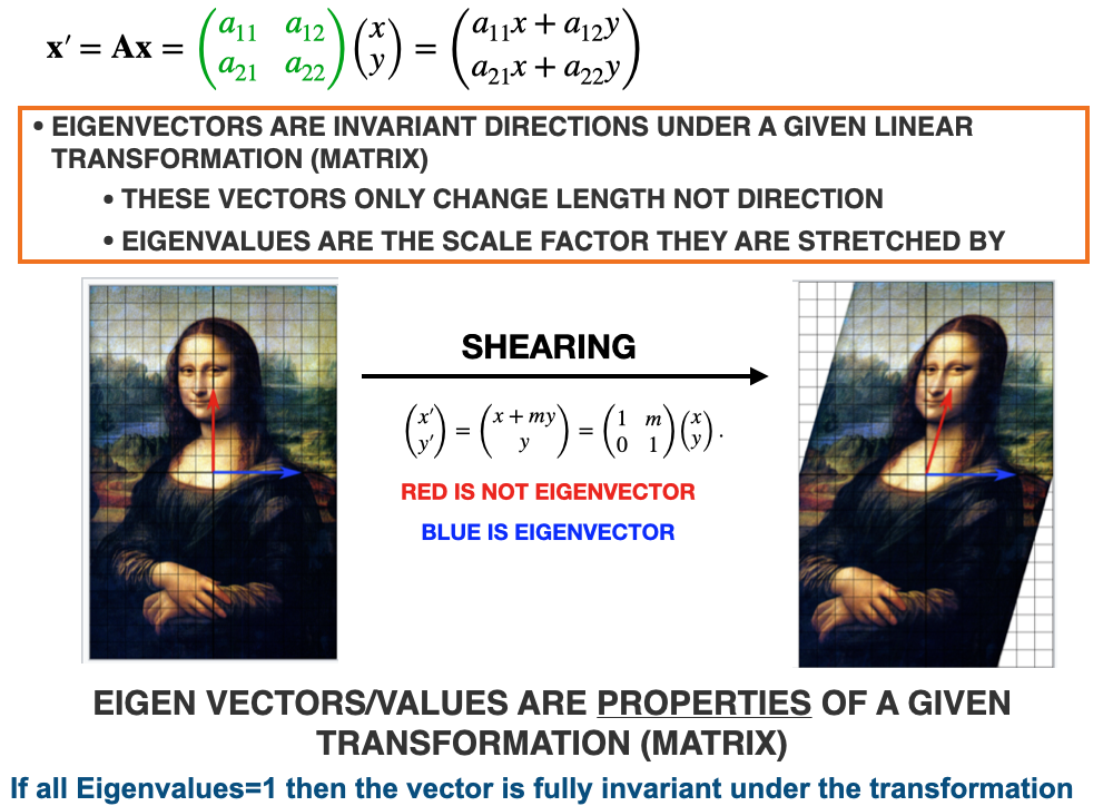
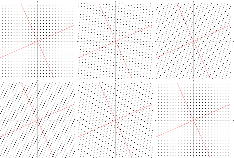
Set up \((A - \lambda I)\mathbf{x} = \mathbf{0}\): what scalars \(\lambda\) make \(A\) act like pure stretching?
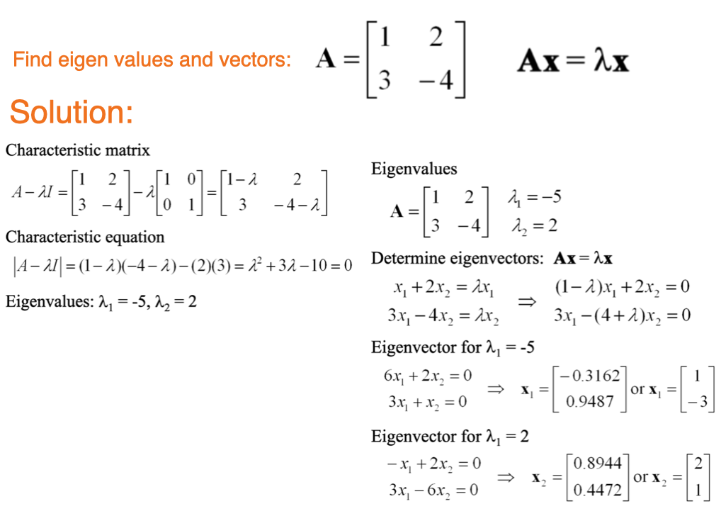
Find eigenvalues via \(\det(A - \lambda I) = 0\): a nonzero solution exists only if \(A - \lambda I\) is singular
\[A \text{ invertible} \iff \det(A) \neq 0 \iff A\mathbf{x} = \mathbf{0} \text{ has only } \mathbf{x} = \mathbf{0}\]
\[\det(A - \lambda I) = 0 \iff (A - \lambda I) \text{ singular} \iff (A-\lambda I)\mathbf{x} = \mathbf{0} \text{ has a nonzero solution}\]
Find eigenvectors by substituting each \(\lambda\) back: the null space of \(A - \lambda I\) reveals which directions are purely stretched
Interpret each \((\lambda, \mathbf{x})\) pair: \(\mathbf{x}\) is a direction \(A\) leaves invariant, scaled by \(\lambda\)
A right eigenvector is a direction that \(A\) merely stretches when acting on column vectors from the left \((A \mathbf{x}=\lambda \mathbf{x})\), while a left eigenvector is a row vector that gets stretched when it acts on \(A\) from the left ( \(\mathbf{y}^{\top} A=\lambda \mathbf{y}^{\top}\) ), same eigenvalues, just the matrix acting from opposite sides.
Running example \(A = \begin{pmatrix} 2 & 1 \\ 0 & 3 \end{pmatrix}\), with eigenvalues \(\lambda = 2, 3\)
Right eigenvectors (the usual case)
\[A\mathbf{x} = \lambda \mathbf{x} \quad\rightarrow\quad \begin{pmatrix} 2 & 1 \\ 0 & 3 \end{pmatrix}\begin{pmatrix} 1 \\ 1 \end{pmatrix} = \begin{pmatrix} 3 \\ 3 \end{pmatrix} = 3\begin{pmatrix} 1 \\ 1 \end{pmatrix}\]
Left eigenvectors
\[\mathbf{y}^\top A = \lambda \mathbf{y}^\top \quad\rightarrow\quad \begin{pmatrix} 0 & 1 \end{pmatrix}\begin{pmatrix} 2 & 1 \\ 0 & 3 \end{pmatrix} = \begin{pmatrix} 0 & 3 \end{pmatrix} = 3\begin{pmatrix} 0 & 1 \end{pmatrix}\]
Key facts
The characteristic polynomial \(\det(A - \lambda I)\) is always degree \(n\) for an \(n \times n\) matrix, giving exactly \(n\) eigenvalues (counting multiplicity, over \(\mathbb{C}\)). One stretching direction per dimension of the space.
Notice that there are \(n\) eigenvalues and \(n\) eigenvectors, one per dimension of the space.
IMPORTANT: Whenever you encounter a well-defined, mathematically meaningful square matrix—especially one with a clear real-world interpretation—it makes sense to analyze its eigenvectors. Examples include the adjacency matrix, covariance matrix, and others.
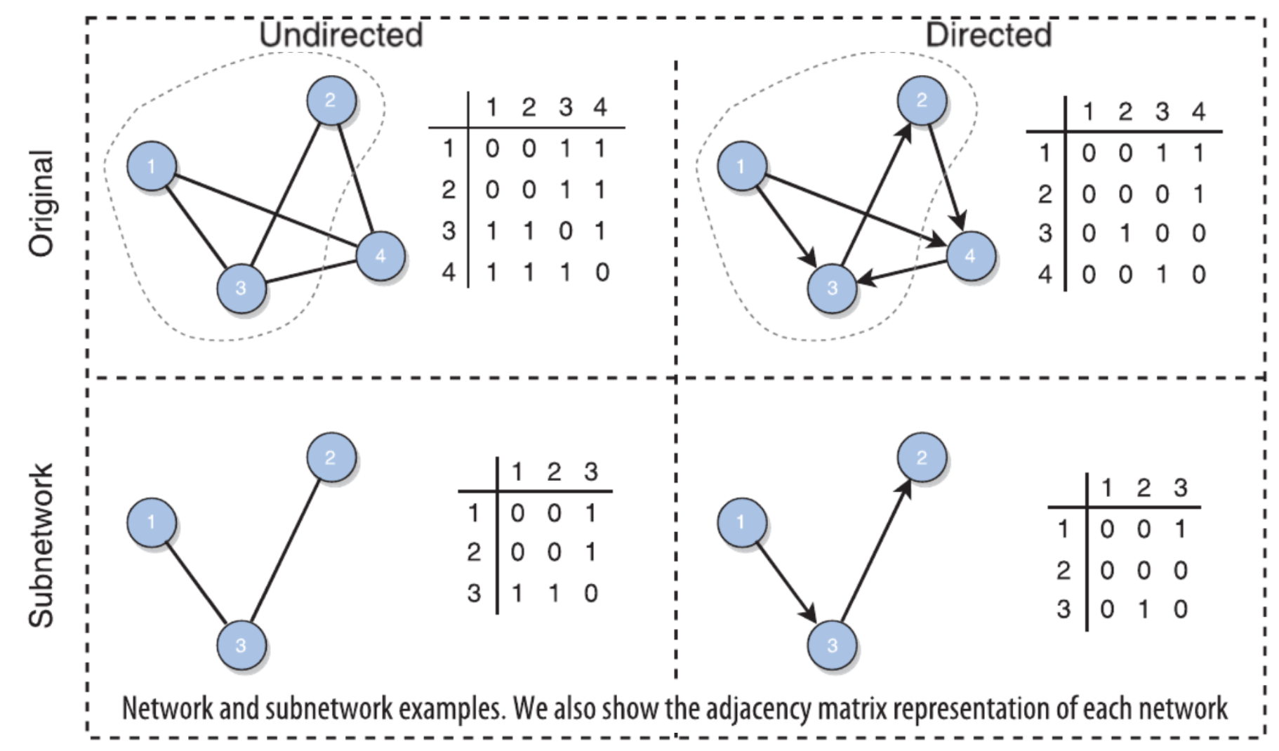
Eigen-centrality is a prestige score which measures the node’s influenceA high Eigen-centrality means the node is connected to many nodes with high scores.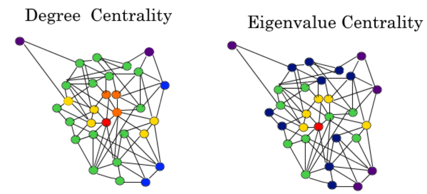
For a network with \(n\) nodes, the adjacency matrix \(A\) is \(n \times n\), and the eigenvector equation is:
\[A\mathbf{x} = \lambda \mathbf{x}, \quad \mathbf{x} \in \mathbb{R}^n\]
Intuition: the eigenvector lives in “node space”, each axis corresponds to a node, and the eigenvector assigns a score along each axis simultaneously, subject to the self-consistency condition across the whole network.
Core idea: a node is important if it is connected to other important nodes, importance is self-referential.
Setup: let \(x_i\) be the centrality of node \(i\). We want each node’s score to be proportional to the sum of its neighbors’ scores:
\[x_i \propto \sum_{j \in \mathcal{N}(i)} x_j \quad \rightarrow \quad \mathbf{x} \propto A\mathbf{x} \quad \rightarrow \quad A\mathbf{x} = \lambda \mathbf{x}\]
This is a self-consistency condition: we seek a centrality assignment where every node’s score is simultaneously explained by its neighbors’ scores, which are explained by their neighbors, and so on.
This is exactly what the eigenvector equation captures: the one centrality vector stable under the entire network’s structure.
Let \(A\) be the adjacency matrix of an undirected graph, where \(A_{ij} = 1\) if nodes \(i\) and \(j\) are connected.
The centrality \(x_i\) of node \(i\) is proportional to the sum of its neighbors' centralities
\[ x_i = \frac{1}{\lambda} \sum_{j} A_{ij}, x_j \]
In matrix form, this is an eigenvalue problem
\[ A\mathbf{x} = \lambda \mathbf{x} \]
The Perron–Frobenius Theorem is the mathematical guarantee that this recursive definition yields a valid, stable ranking.
For any strongly connected network (where every node can reach every other node), the theorem guarantees that the matrix \(A\):
Without outgoing edges to recirculate influence, the matrix loses its mathematical “irreducibility.” Consequently, the Perron–Frobenius guarantees collapse, and the centrality scores of entire clusters can drain away, dropping to zero. This fatal flaw is why PageRank introduces a “damping factor” (random teleportation)—it artificially restores strong connectivity so the Perron–Frobenius theorem can function properly.
eigenvector_centrality(G, max_iter=100, tol=1e-06, nstart=None, weight=None)
import networkx as nx
import numpy as np

# CREATE-1
G=nx.complete_graph(3)

# CREATE-2
# G = nx.DiGraph()
# G = nx.Graph()
# G.add_nodes_from([0,1,2,3,4])
# G.add_edges_from([(0, 1), (0, 2), (0,3), (0,4),(1,0),(2,3)])

# DRAW
nx.draw(G)

# ADJACENCY MATRIX
A=nx.adjacency_matrix(G).todense()
print("Adjacency matrix\n",A)

# METHOD-1: NETWORKX EIGENVECTOR_CENTRALITY
print("\nEIGENVECTOR_CENTRALITY:\n",nx.eigenvector_centrality(G))

# METHOD-2: COMPUTE FROM "SCRATCH"
print("EIGENVALUES:",np.linalg.eig(A)[0])
eVect=np.array(np.linalg.eig(A)[1])
print("\nEIGENVECTORS:\n",np.round(eVect,4))
print("LENGTH OF EIGEN VECTORS:",
np.sqrt(np.sum((eVect)**2,axis=0))**0.5)
Adjacency matrix
[[0 1 1]
[1 0 1]
[1 1 0]]
EIGENVECTOR_CENTRALITY:
{0: 0.5773502691896258, 1: 0.5773502691896258, 2: 0.5773502691896258}
EIGENVALUES: [-1. 2. -1.]
EIGENVECTORS:
[[-0.8165 0.5774 0.2265]
[ 0.4082 0.5774 -0.7926]
[ 0.4082 0.5774 0.5661]]
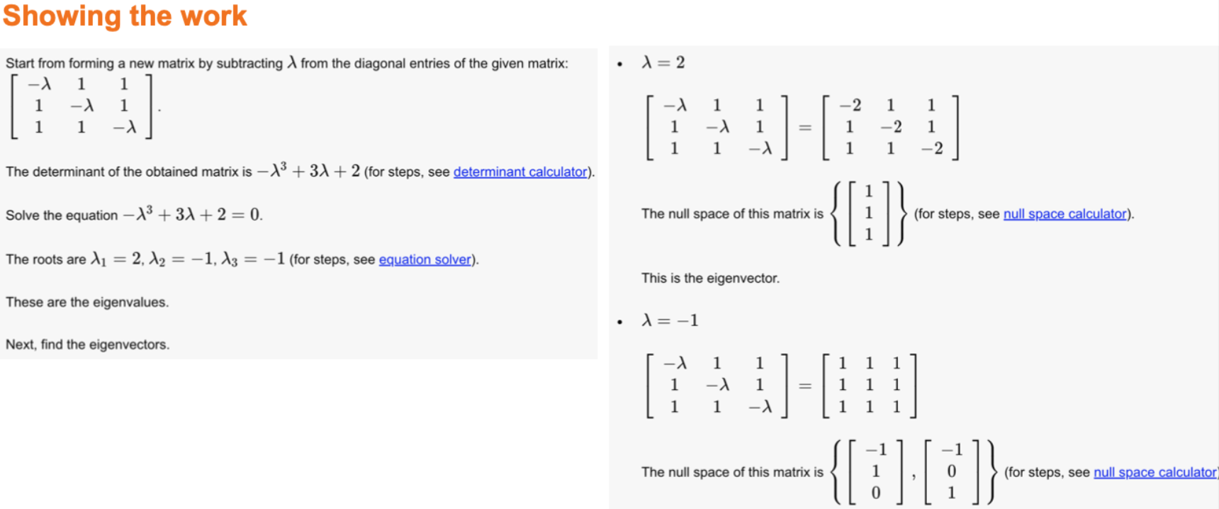
LENGTH OF EIGEN VECTORS: [1. 1. 1.]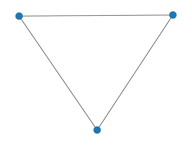
Source: https://www.emathhelp.net/en/calculators/linear-algebra/eigenvalue-and-eigenvector-calculator/
Note: 1/sqrt(3)=0.577350

# Generate graph
import networkx as nx
G = nx.DiGraph()
G.add_nodes_from([0,1,2,3,4])
G.add_edges_from([(0, 1), (0, 2), (0,3), (0,4),(1,0),(2,3)])
nx.draw(G,with_labels=True)


# ADJACENCY MATRIX
A=nx.adjacency_matrix(G).todense().T #TRANSPOSE MAKES IT IN-DEGREE ORIENTS ROWS=IN
print("Adjacency matrix\n",A)

# METHOD-1: NETWORKX EIGENVECTOR_CENTRALITY
print("\nEIGENVECTOR_CENTRALITY:\n",nx.eigenvector_centrality(G))

# METHOD-2: COMPUTE FROM "SCRATCH"
print("EIGENVALUES:",np.linalg.eig(A)[0])
eVect=np.array(np.linalg.eig(A)[1])
print("\nEIGENVECTORS:\n",np.round(eVect,4))
print("LENGTH OF EIGEN VECTORS:",
np.sqrt(np.sum((eVect)**2,axis=0))**0.5)
Adjacency matrix
[[0 1 0 0 0]
[1 0 0 0 0]
[1 0 0 0 0]
[1 0 1 0 0]
[1 0 0 0 0]]
EIGENVECTOR_CENTRALITY:
{0: 0.35355406494349306, 1: 0.35355406494349306, 2: 0.35355406494349306, 3: 0.7071054324835365, 4: 0.35355406494349306}
EIGENVALUES: [ 0. 0. 0. 1. -1.]
EIGENVECTORS:
[[ 0. 0. 0. 0.3536 -0.5 ]
[ 0. 0. 0. 0.3536 0.5 ]
[ 0. 0. 0. 0.3536 0.5 ]
[ 1. -1. 0. 0.7071 0. ]
[ 0. 0. 1. 0.3536 0.5 ]]
LENGTH OF EIGEN VECTORS: [1. 1. 1. 1. 1.]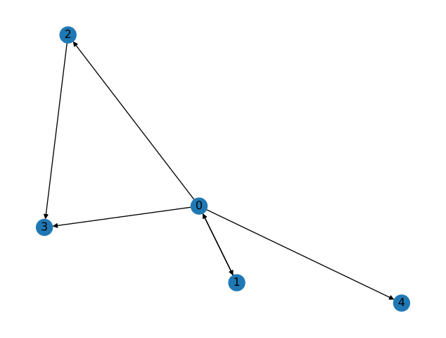
Eigencentrality works best for undirected graphs because they always yield a symmetric matrix with a clear, guaranteed principal eigenvector, whereas directed graphs can produce asymmetric matrices where centrality scores fail to properly propagate backward from “dead ends” or sinks.
nx.eigenvector_centrality), and the basis for Katz centrality and PageRank