The GCN Architecture
Graph convolutional networks
Motivating example
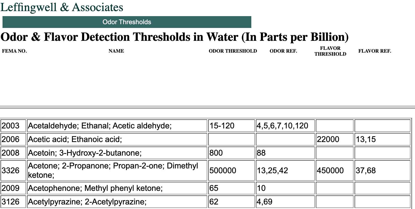
Leffingwell Odor Dataset
Overview of types of GNNs
- Graph Convolutional Networks (GCNs):
- Generalize the convolution operation to graph structures.
- Aggregate features from neighboring nodes to update each node’s representation.
- Example: Kipf and Welling’s GCN.
- Message Passing Neural Networks (MPNNs):
- A general framework where nodes communicate by passing messages along edges.
- Update node features by aggregating incoming messages from neighbors.
- Example: Gilmer et al.’s MPNN.
- Graph Attention Networks (GATs):
- Use attention mechanisms to assign different weights to neighboring nodes.
- Allow the network to focus on the most relevant parts of the graph.
- Example: Veličković et al.’s GAT.
- Spectral-based GNNs:
- Operate in the spectral domain using the graph Laplacian.
- Involve complex computations, often making them less scalable.
- Example: Bruna et al.’s Spectral Networks. ->
- Spatial-based GNNs:
- Operate directly on the graph structure in the spatial domain.
- Aggregate information from local neighborhoods.
- Example: GraphSAGE (Graph Sample and Aggregation).
- Graph Recurrent Networks (GRNs):
- Use recurrent neural network architectures to process graph data.
- Suitable for capturing dependencies in sequential data represented as graphs.
- Example: GGNN (Gated Graph Neural Network).
- Graph Autoencoders:
- Unsupervised models that learn to encode graph data into low-dimensional embeddings and then decode them back.
- Used for tasks like graph reconstruction and link prediction.
- Example: Graph Autoencoder (GAE) and Variational Graph Autoencoder (VGAE).
- GraphSAGE:
- A framework for inductive representation learning on large graphs.
- Aggregates feature information from a node’s local neighborhood.
- Example: Hamilton et al.’s GraphSAGE.
Dataset
- Our playground shows a graph-level prediction task with small molecular graphs
Leffingwell Odor Dataset: Composed of molecules with associated odor percepts (labels).- Predicting the relation of a molecular structure (graph) to its smell (target)
- Consider only a single binary label per molecule, classifying if a molecular graph smells “pungent” (e.g. garlic,peppermint, or mustard) or not
Data: Represent each molecule as a graph, atoms are nodes containing a one-hot encoding for atomic identity (Carbon, Nitrogen, Oxygen, Fluorine) and bonds are edges containing a bond type one-hot encoding (single, double, triple or aromatic).
GNN Model
Build our model using sequential GNN layers, followed by a linear model with a sigmoid activation for classification.
The
design spacefor our GNN has many hyper-parameters that can customize the model:The number of GNN layers, also called the depth.
The dimensionality of each attribute when updated. The update function is a 1-layer MLP with a relu activation function and a layer norm for normalization of activations.
The aggregation function used in pooling: max, mean or sum.
The graph attributes that get updated, or styles of message passing: nodes, edges and global representation. We control these via boolean toggles (on or off).
A
baseline modelwould be a graph-independent GNN (all message-passing off) which aggregates all data at the end into a single global attribute. Toggling on all message-passing functions yields a GraphNets architecture.
Results
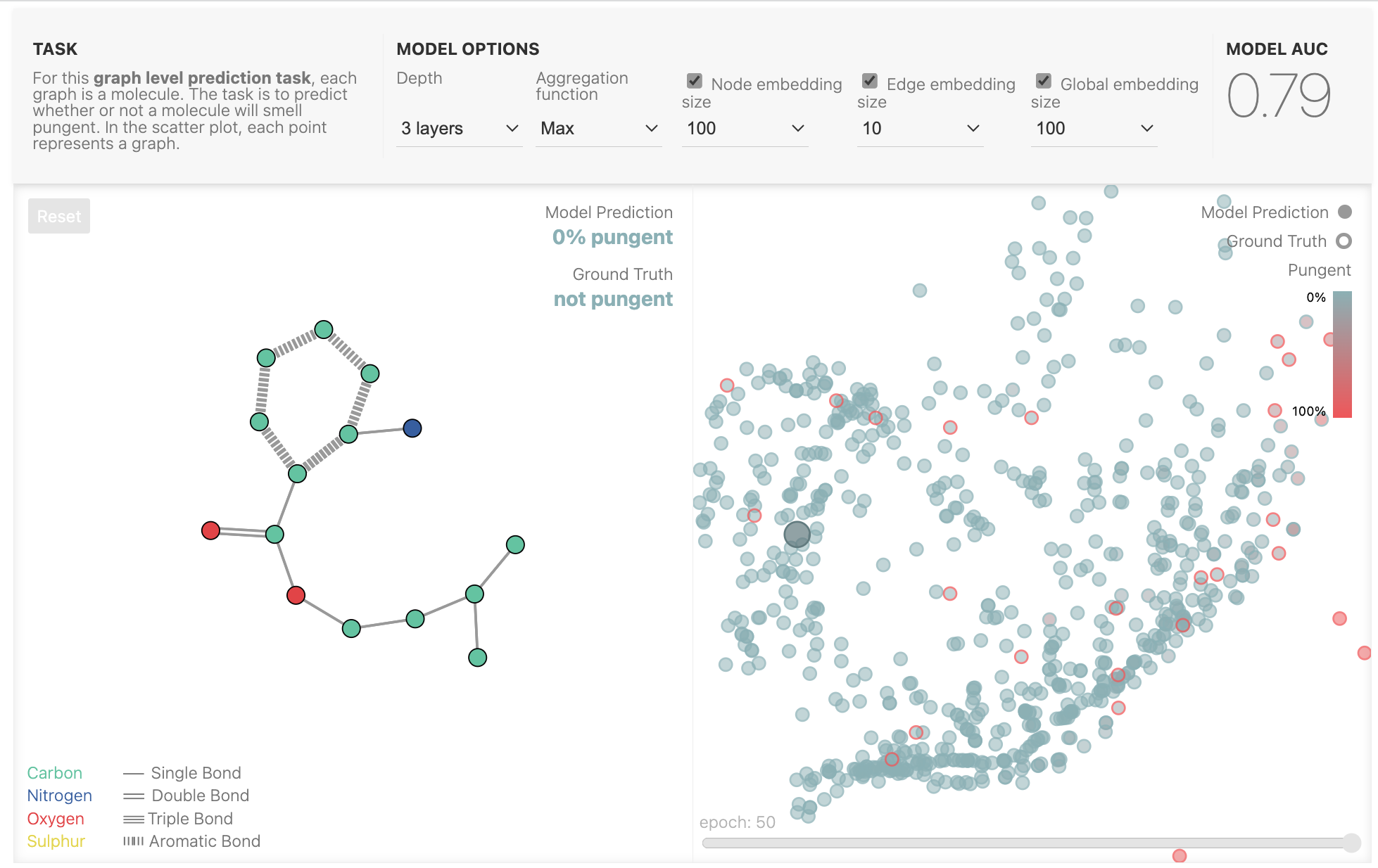
For this graph level prediction task, each graph is a molecule. The task is to predict whether or not a molecule will smell pungent. In the scatter plot, each point represents a graph.
You can edit the molecule to see how the prediction changes, or change the model params to load a different model.
Select a different molecule in the scatter plot.
Graph Convolutions
Big picture overview
Motivation
- Graph convolutions update node representation using structural connectivity info in \(A\)
- GCNs leverage the graph structure to learn meaningful representations.
- Numerous kinds of graph convolutions exist (active area of research)
- Graph convolution: Extend the concept of convolutions to non-Euclidean domains.
- Key idea: Aggregate information from a node’s neighbors to compute its updated representation.
General idea
Recall image CNN properties
- Convolutions in Image Processing:
- Effective due to parameter independence from input size.
- 3x3 filters applicable to various image resolutions.
- Properties: shift-invariance, locality, hierarchy.
- Convolutional Approach for Images and Graphs:
- Both leverage locality priors.
- Images: locality in 2D space.
- Graphs: structural locality; closer nodes are more related.
Dealing with data of variable size
- Convolutional approaches are beneficial for graphs as they use a fixed parameter set for graphs of different sizes.
- This fixed parameter set is more critical for graphs than images.
- Many image datasets have a fixed resolution, allowing fully connected approaches, unlike graph datasets with varying sizes.
- Image convolutional operators are standardized, whereas graph convolutions are diverse and actively researched.
Weight Sharing: The CNN Analogy
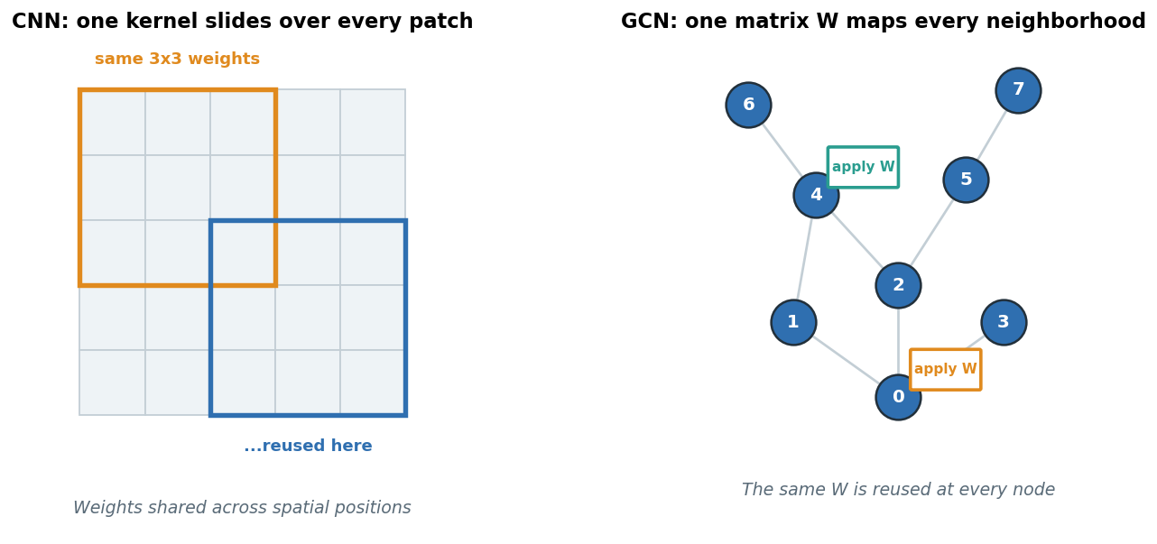
- CNN: one small kernel slides across an image: the same weights reused at every position.
- GCN: one matrix
Wis applied at every node’s neighborhood: the same weights everywhere. - Why it’s powerful:
- Few parameters: model size is independent of how many nodes/pixels there are.
- Generalizes: a pattern learned in one region works in another.
- Permutation-equivariant: relabeling nodes just relabels outputs; the graph has no fixed “first” node.
The mental model of a GCN
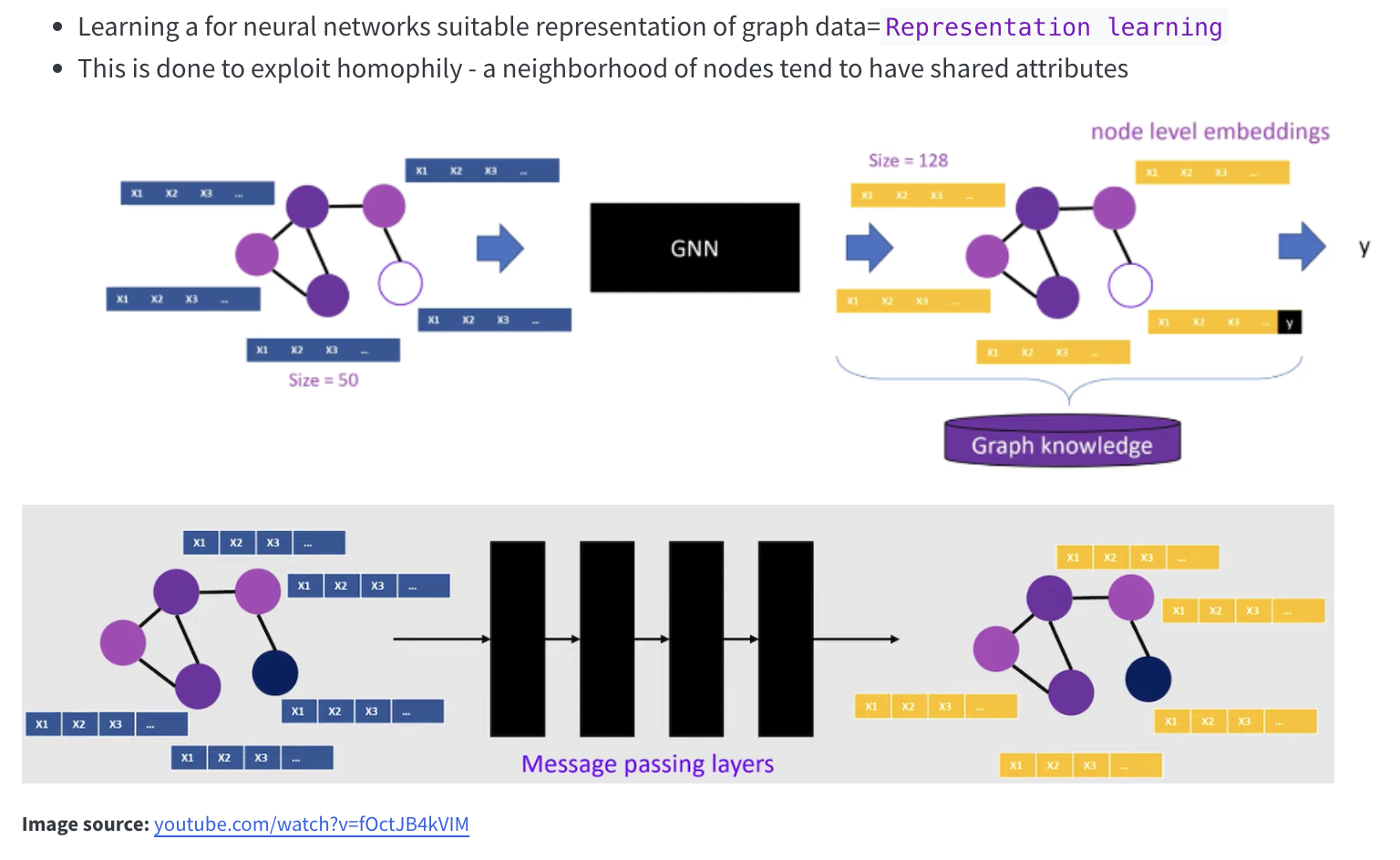
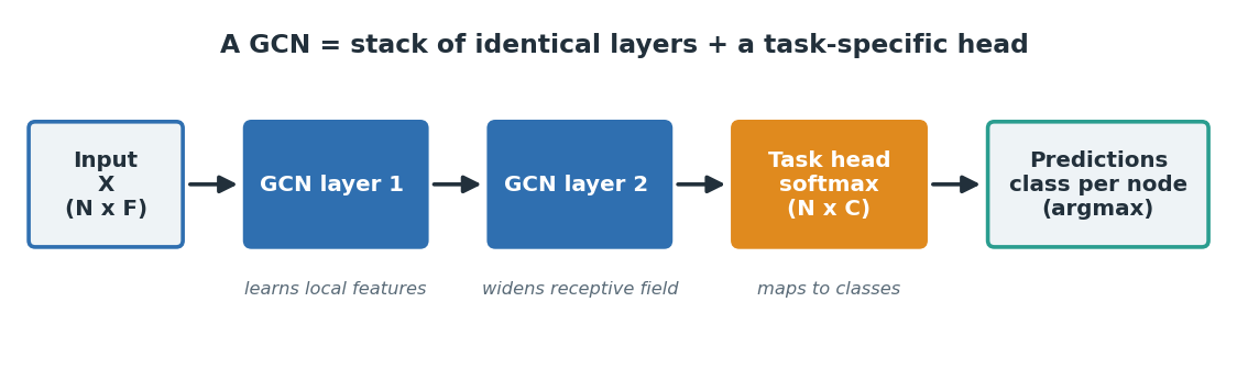
- A Graph Convolutional Network (GCN) is just a stack of identical layers plus a small task head.
- Each layer does one thing: mix each node with its neighbors, then re-express the result.
- We already know the single-layer rule: today we zoom out to the whole network.
- By the end you should see a GCN the way you see a CNN: a module you drop into a pipeline.
The full assembly line:
Here we use node level classification as an example, but below we will see how this pipeline can be used for different learning tasks.
Three steps, applied to every node
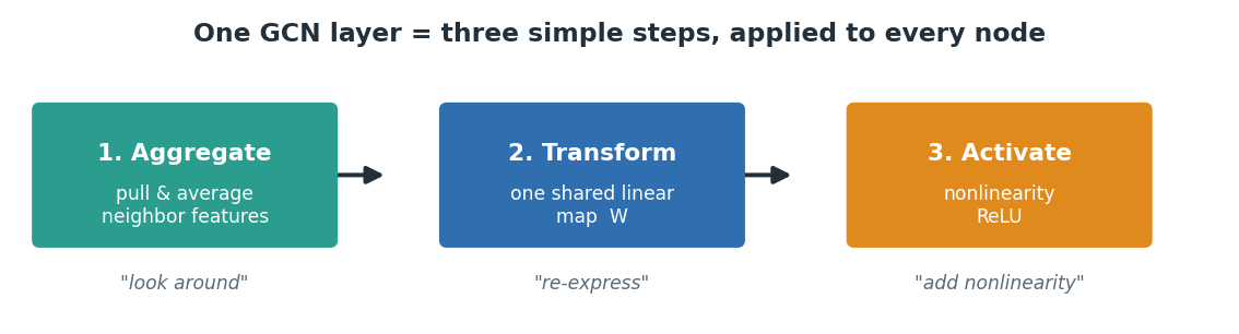
A single layer is the composition of three familiar operations:
- Aggregate: each node pulls in and averages its neighbors’ feature vectors (normalized).
- Transform: multiply by one shared weight matrix
W(a linear re-expression). - Activate: apply a nonlinearity like
ReLU(so stacked layers aren’t just one big linear map).
That’s the whole layer. Everything else is bookkeeping.
Stacking Layers = a \(k\)-Hop Receptive Field
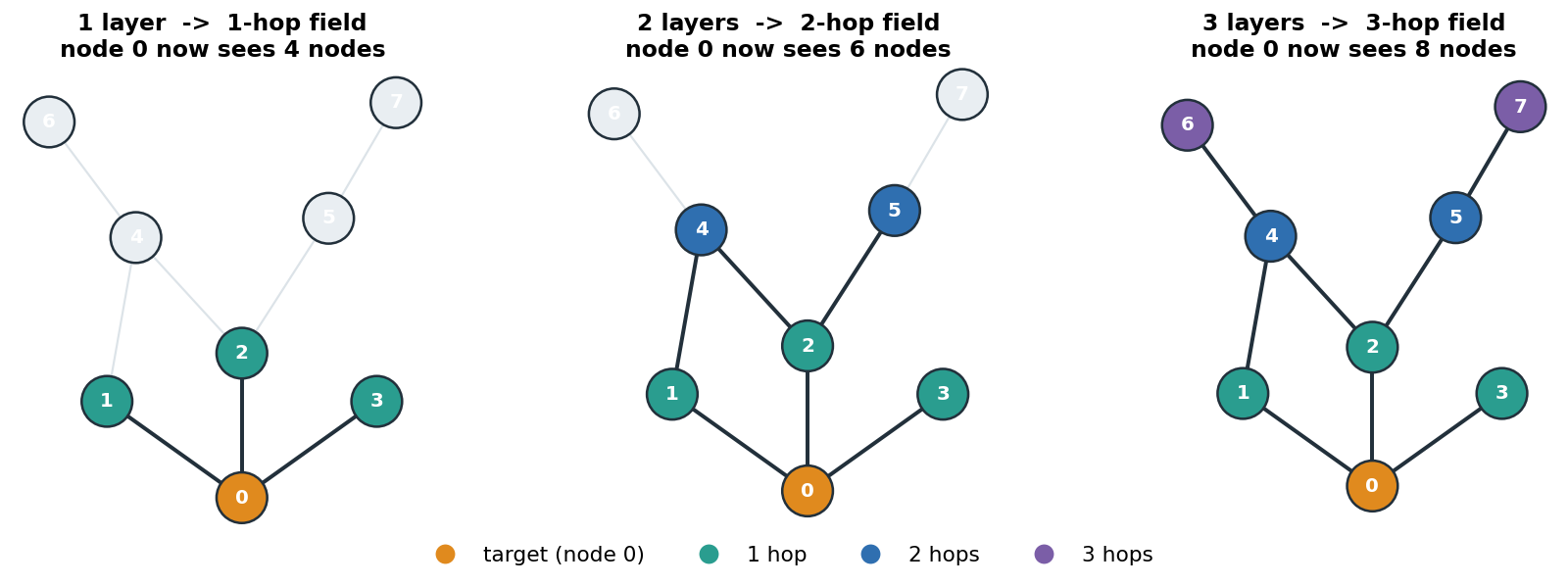
- One layer sees one hop: so we stack them
- 1 layer: a node blends with its direct neighbors → info travels 1 hop.
- 2 layers: neighbors have already blended with their neighbors → info travels 2 hops.
- \(k\) layers → each node’s output depends on everything within \(k\) hops: its \(k\)-hop receptive field.
- Same principle as a CNN: deeper = wider field of view, just measured in graph hops not pixels.
Alternative visualization
Example-1: A simple Graph Convolution
Textbook example
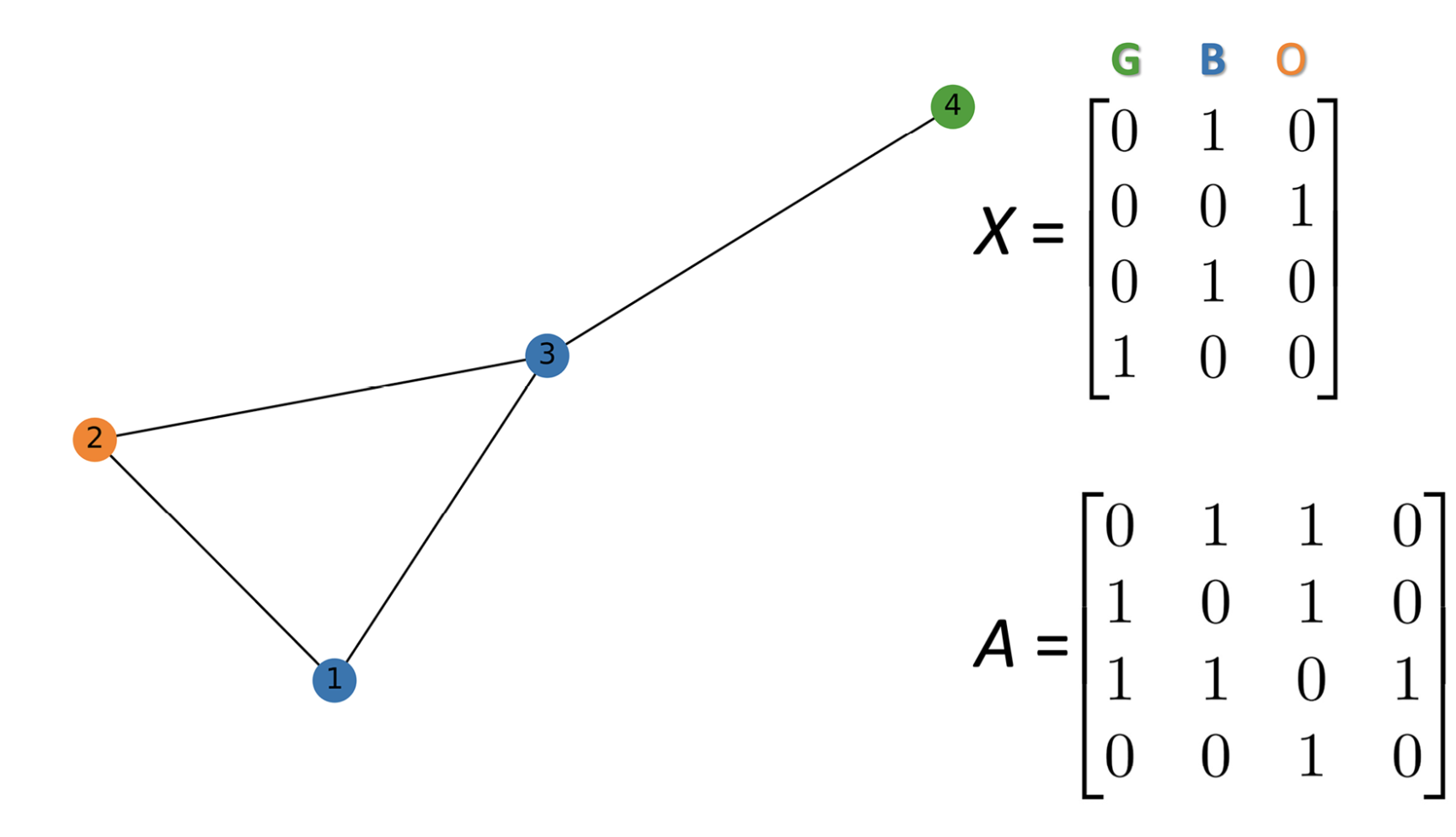
Data: Graph representation
- Undirected graph with \(n\) nodes and \(n \times n\) adjacency matrix \(\boldsymbol{A}\)
- \(n \times f_{\text {in }}\) node feature matrix \(\boldsymbol{X}\)
- Only feature is a one-hot representation of each node’s color-green (G), blue (B), or orange (O).
Aside: Setting up this graph in NetworkX
- NetworkX is a Python package for the creation, manipulation, and study of the structure, dynamics, and functions of complex networks.
- We can use it to create the graph and get the adjacency matrix.
Adjacency matrix:
 [[0 1 1 0]
 [1 0 1 0]
 [1 1 0 1]
 [0 0 1 0]]
Visualize the graph
Node feature matrix:
 [[0. 1. 0.]
 [0. 0. 1.]
 [0. 1. 0.]
 [1. 0. 0.]]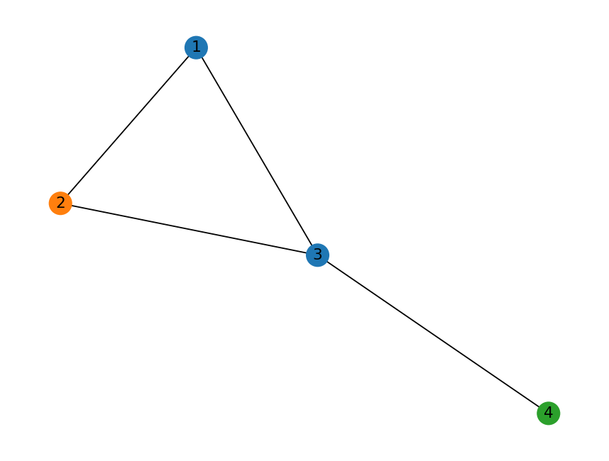
Convolution Formula
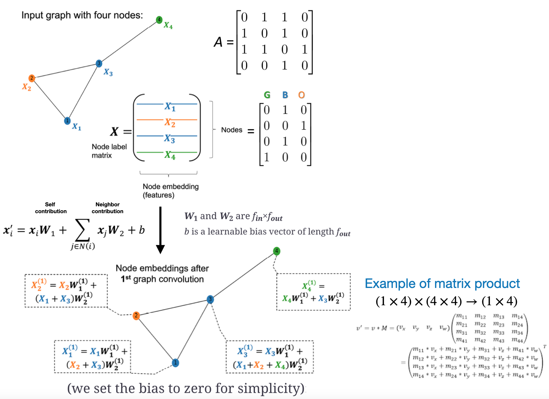
- Graph convolutions update the embeddings at each node based on the embeddings of their neighbors and themselves.
- The following is ONE possible spatial graph convolution (there are others)
\[ \boldsymbol{x}_i^{\prime}=\boldsymbol{x}_i \boldsymbol{W}_1+\sum_{j \in N(i)} x_j \boldsymbol{W}_2+b \]
- \(\boldsymbol{x}_i^{\prime}\) –> updated embedding for node \(i\);
- Recall \(\mathbf x_i\) is size \(n \times f_{\text {in }}=(4 \times 3)\)
- Recall: each row of X –> corresponding node information embedding vector
- \(\boldsymbol{W}_1\) and \(\boldsymbol{W}_2\) are \(f_{\text {in }} \times f_{\text {out }}\) matrices of learnable filter weights;
- \(b\) is a learnable bias vector of length \(f_{out}\).
Graph convolution
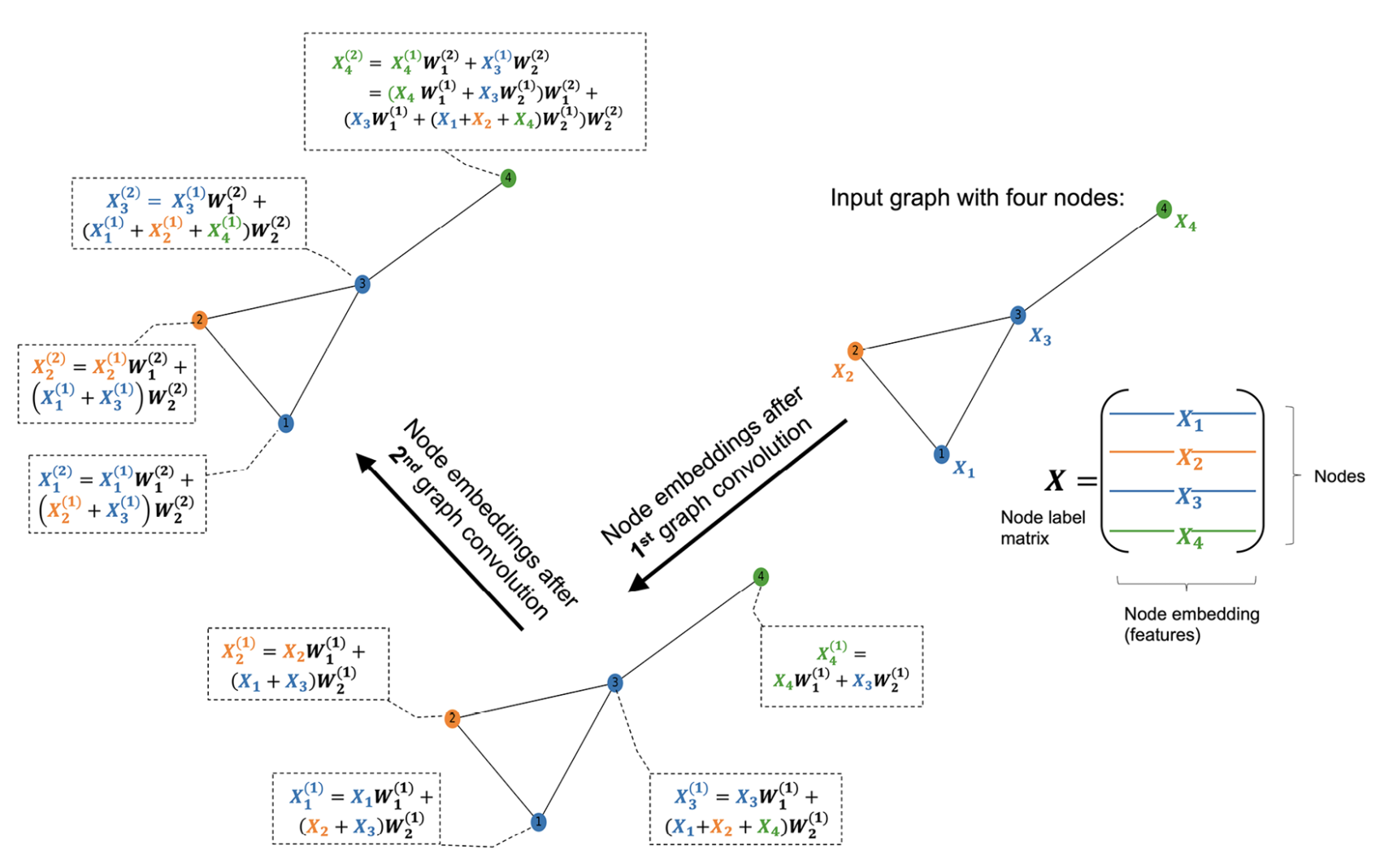
- A single convolution is insufficient to capture a relationship between a node and another node located many edges away.
Aside: np.dot vs np.matmul
- NOTE:
np.dot()in NumPy performs the dot product of two arrays.- For 1D vectors, it computes the
inner product; - For 2D matrices, it performs
matrix multiplication.
- For 1D vectors, it computes the
notice how the following are equivalent
dot:
 [[6 4]
 [6 4]]
matmul:
 [[6 4]
 [6 4]]
Weight matrices
- The two weight matrices can be considered filter banks, where each column is an individual filter.
- Filter expects that
locality prioron graph holds.- A single convolution will not capture long range correlations relationships (distance>2).
- Stacking convolutions captures more distant relationships
Let make some random matrices to “act as” the weight matrices.
f_in: 3
f_out: 6
W_1: (3, 6)
W_2: (3, 6)
b: (1, 6)
W_1:
 [[0.43599 0.02593 0.54966 0.43532 0.42037 0.33033]
 [0.20465 0.61927 0.29965 0.26683 0.62113 0.52914]
 [0.13458 0.51358 0.18444 0.78534 0.85398 0.49424]]
W_2:
 [[0.84656 0.07965 0.50525 0.06529 0.42812 0.09653]
 [0.12716 0.59675 0.22601 0.10695 0.22031 0.34983]
 [0.46779 0.20174 0.64041 0.48307 0.50524 0.38689]]
b:
 [[0.79364 0.58    0.1623  0.70075 0.96455 0.50001]]
Batch implementation
- A batch implementation applies the formula for all samples (nodes) all at once
\[x_i^{\prime}=x_i W_1+\sum_{j \in N(i)} x_j W_2+b\]
This is a batch implementation, if we multiply on the left by X, we apply the transformation the feature vectors of all nodes.
- We discussed this earlier in the context of MLP
Summation implementation of convolution
Lets first implement the sum of the weighted inputs for each node.
\[x_i^{\prime}=x_i W_1+\sum_{j \in N(i)} x_j W_2+b\]
NODE-0
node 0: [0. 1. 0.]
X[i].shape: (3,), W_1.shape: (3, 6)
self_update: [0.20465 0.61927 0.29965 0.26683 0.62113 0.52914], shape: (6,)
neighbor_update: [0.59495 0.79849 0.86642 0.59002 0.72555 0.73672], shape: (6,)
output:
 [[1.59324 1.99776 1.32837 1.5576  2.31123 1.76587]
 [1.18254 2.28708 0.79876 1.69999 2.25915 1.69391]
 [2.4398  2.07741 1.83362 1.62289 2.73935 1.8624 ]
 [1.35679 1.20268 0.93797 1.24302 1.60523 1.18017]]
(4, 6)
Matrix implementation of convolution
We can get the exact same result in a much more compact and efficient manner by using matrix multiplication.
A:
 [[0 1 1 0]
 [1 0 1 0]
 [1 1 0 1]
 [0 0 1 0]]
W_1: (3, 6)
W_2: (3, 6)
(4, 3) (3, 6) (4, 6)
[[1.59324 1.99776 1.32837 1.5576  2.31123 1.76587]
 [1.18254 2.28708 0.79876 1.69999 2.25915 1.69391]
 [2.4398  2.07741 1.83362 1.62289 2.73935 1.8624 ]
 [1.35679 1.20268 0.93797 1.24302 1.60523 1.18017]]
Multiple convolutional layers
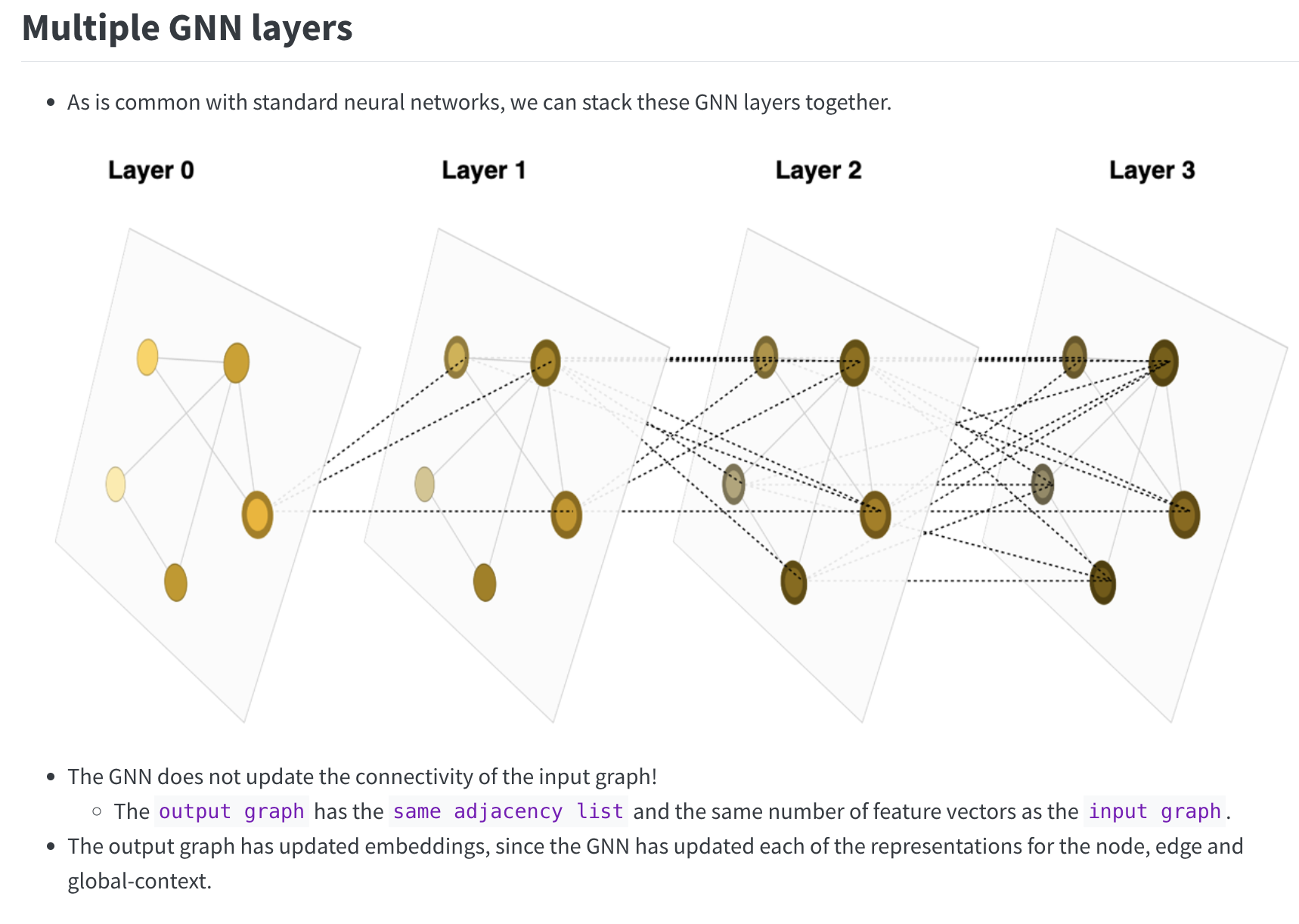
- We can stack multiple convolutions to capture more distant relationships in the network
Mathematical notations
Let’s see how these equations are generalized into matrix form.
GCN: Alternative summation formalism
\[ \mathbf{h}_i^{(k+1)}=\sigma\left(\sum_{j \in \mathcal{N}(i) \cup\{i\} } \frac{1}{c_{i j}} \mathbf{W}^{(k)} \mathbf{h}_j^{(k)}\right) \]
Explanation of Components:
- Node Features:
- \(\mathbf{h}_i^{(k)}\) : The feature vector of node \(i\) at the \(k\)-th layer.
- \(\mathbf{h}_i^{(k+1)}\) : The updated feature vector of node \(i\) at the \((k+1)\)-th layer.
- Neighborhood Aggregation:
- \(\mathcal{N}(i)\) : The set of neighbors of node \(i\).
- The summation aggregates information from node \(i\) ’s neighbors as well as the node itself.
- Normalization Term:
- \(c_{i j}\) : A normalization coefficient, often based on the graph’s structure (e.g., the degree of nodes). For instance, in
- Graph Convolutional Networks (GCNs), this is typically:
- \(c_{i j}=\sqrt{\operatorname{deg}(i) \cdot \operatorname{deg}(j)}\)
- where \(\operatorname{deg}(i)\) is the degree of node \(i\).
- Learnable Parameters:
- \(\mathbf{W}^{(k)}\) : A learnable weight matrix at the \(k\)-th layer.
- Nonlinearity:
- \(\sigma\) : A nonlinear activation function (e.g., ReLU, Sigmoid).
GCN: Alternative matrix formalism
Layer-Wise Propagation:
- In GCNs, the node feature update is typically:
\[ \mathbf{H}^{(k+1)}=\sigma\left(\hat{\mathbf{D}}^{-\frac{1}{2}} \hat{\mathbf{A}} \hat{\mathbf{D}}^{-\frac{1}{2}} \mathbf{H}^{(k)} \mathbf{W}^{(k)}\right) \]
- H: Matrix of node representations \(\left(\mathbf{h}_u\right)\).
- \(\mathbf{X}\) : Matrix of node features \(\left(\mathbf{x}_u\right)\).
- \(\sigma(\cdot)\) : Activation function (e.g., ReLU).
- \(\tilde{\mathbf{A}}\) : Adjacency matrix with added self-loops \((\mathbf{A}+\mathbf{I})\).
- \(\tilde{\mathbf{D}}\) : Degree matrix corresponding to \(\tilde{\mathbf{A}}\).
Graph Normalization
- Graph Normalization:
- Compute \(\tilde{\mathbf{A}}=\mathbf{A}+\mathbf{I}\), where \(\mathbf{I}\) is the identity matrix.
- Define \(\tilde{\mathbf{D}}_{i i}=\sum_{j \in V} \tilde{A}_{i j}\).
- Use normalized adjacency \(\tilde{\mathbf{D}}^{-\frac{1}{2}} \tilde{\mathbf{A}} \tilde{\mathbf{D}}^{-\frac{1}{2}}\) to ensure eigenvalues lie in \([0,1]\), preventing numerical instabilities.
- Purpose of Normalization:
- Avoid exploding or vanishing gradients during training.
- Ensure stable learning dynamics.
- Practical Implication:
- Weighted graphs can be incorporated by encoding edge weights in \(\mathbf{A}\).
Step 1: Normalized neighbor aggregation
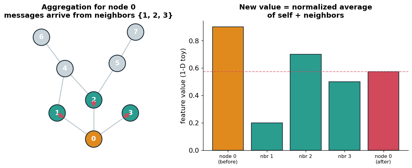
- Each node’s new value is a weighted average of itself + its neighbors.
- “Normalized” = we divide out node degrees so high-degree nodes don’t dominate (next section).
- Intuition: “describe me by the company I keep.”
- Left: messages flow into node 0 from
{1, 2, 3}. Right: the values get blended.
Steps 2 & 3: Transform, then activate
- Transform: the aggregated vector is multiplied by
W, a matrix learned by gradient descent.Wchanges the feature dimension (e.g.F -> H) and lets the layer emphasize useful directions.- Crucially, the same
Wis used for every node (weight sharing: more soon).
- Activate: apply
ReLUelement-wise.- Without it, two stacked layers \(\hat{A}(\hat{A}XW_1)W_2\) would collapse into a single linear map.
- The layer in one line:
\[H^{(l+1)} = \sigma\!\left(\hat{A}\, H^{(l)}\, W^{(l)}\right)\]
where \(\hat A\) = normalized aggregation, \(W^{(l)}\) = shared weights, \(\sigma\) = ReLU, and \(H^{(0)} = X\).
The Renormalization Trick: Building \(\hat{A}\)
Why raw aggregation breaks
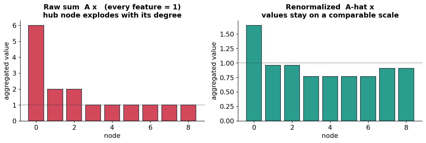
- Naive aggregation = “sum my neighbors’ features,” i.e. multiply features by
A. - Problem: a node with many neighbors gets a huge sum; a node with few gets a tiny one.
- Feature magnitudes then track degree, not content: and they can explode across layers.
- Below: one toy graph, every node’s feature = 1. Raw
A·xblows up at the hub;·xstays tame.
From \(A\) to \(\hat{A}\) in three moves
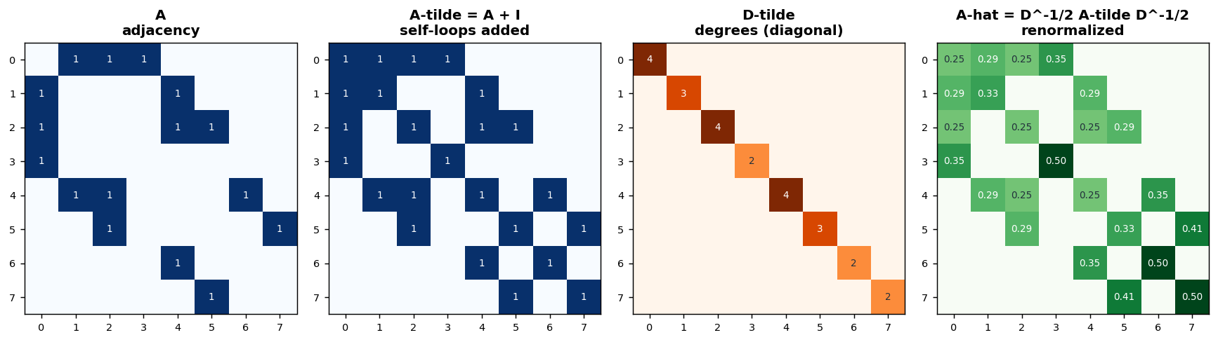
\[\hat{A} = \tilde{D}^{-1/2}\,(A+I)\,\tilde{D}^{-1/2}, \qquad \tilde{A}=A+I\]
- Add self-loops (\(A+I\)): a node should include its own features, not just neighbors’.
- Build \(\tilde D\): the diagonal degree matrix of \(\tilde A\) (each node’s neighbor count, +1 for itself).
- Symmetric normalize (\(\tilde D^{-1/2}\,\tilde A\,\tilde D^{-1/2}\)): scale each edge by both endpoints’ degrees.
Watch the four matrices for our 8-node graph:
What \(\hat{A}\) actually does
- \(\hat A\) is a fixed matrix: it depends only on the graph, not on learnable weights.
- One multiply \(\hat A H\) = “every node simultaneously does one round of normalized neighbor-averaging.”
- Entry \(\hat A_{ij}\) is large when nodes \(i,j\) are connected and both have few neighbors.
- Think of \(\hat A\) as the “who-talks-to-whom, and how loudly” operator, reused in every layer.
The Full Anatomy, End to End
Dimensions flowing through the network
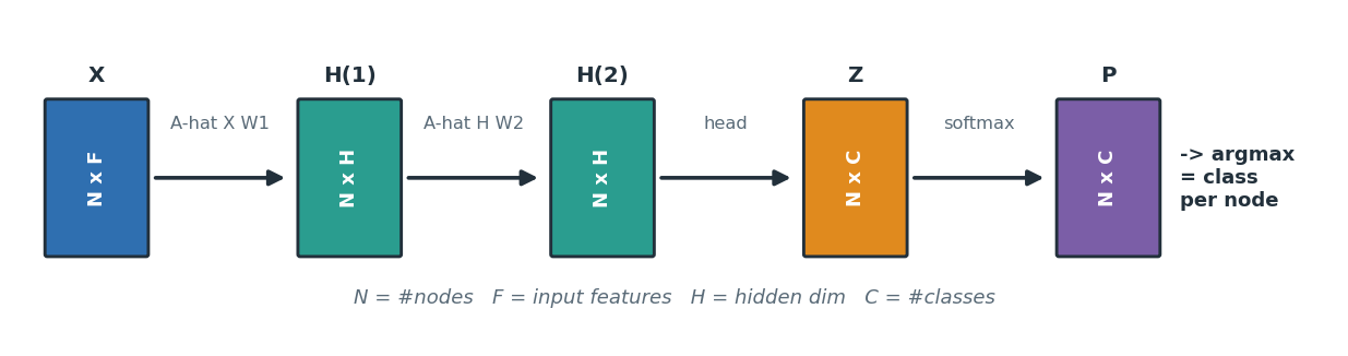
- Track the shapes and the whole model becomes obvious bookkeeping:
X: N × F (nodes × input features)- after layer 1: N × H (H = hidden width, your choice)
- after layer 2: N × H
- logits
Z: N × C (C = number of classes) - probabilities
P: N × C, then argmax → one class per node.
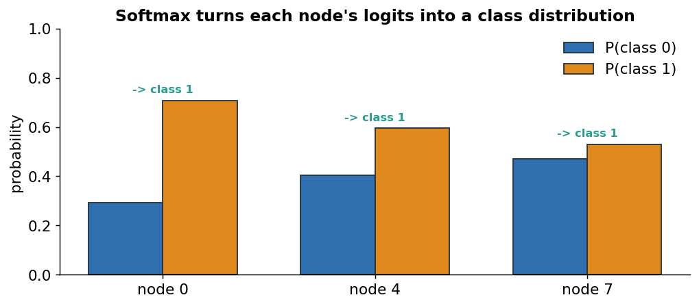
The task head: softmax over node classes
- For node classification, the head is a softmax over the
Clogits of each node. - Output = a probability distribution per node; argmax picks the predicted class.
- Training minimizes cross-entropy on the labeled nodes; gradients flow back into every
W. - Swap the head to change the task (graph-level readout, link scoring, regression, …).
How Deep Should You Go?
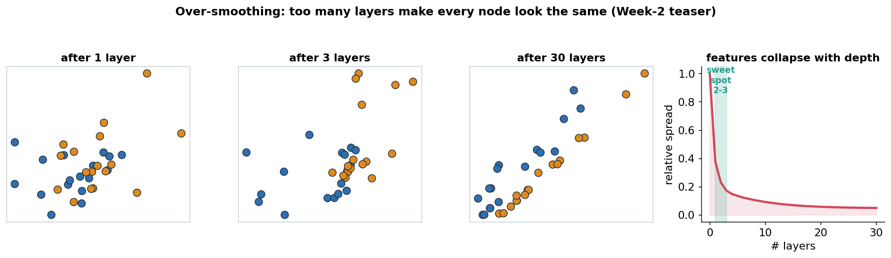
The 2–3 layer rule & over-smoothing
- Deeper GCNs repeatedly average node features: so they slowly become identical.
- Past a few layers, every node’s vector converges toward the same thing → over-smoothing.
- Classes stop being separable, and accuracy drops. The practical sweet spot is 2–3 layers.
- Below (Zachary’s karate club): two communities stay separated early, then collapse by depth 30.
Practical recipe
- Depth: start with 2 layers; try 3 only if the graph is large/sparse and it helps.
- Width: a modest hidden dim (
H = 16–64) is plenty for small benchmarks. - Between layers:
ReLU+dropout; a final softmax head for classification. - Precompute \(\hat A\) once: it never changes during training.
- If deeper must work: residual/skip connections, jumping-knowledge, or
PairNorm(Week 2).
Things to remember
- A layer = aggregate → transform → activate: \(H^{(l+1)} = \sigma(\hat A H^{(l)} W^{(l)})\).
- \(\hat A = \tilde D^{-1/2}(A+I)\tilde D^{-1/2}\) is a fixed operator: normalized neighbor-averaging with self-loops.
- Stacking \(k\) layers = a \(k\)-hop receptive field: deeper sees farther across the graph.
- Weight sharing: the same
W(like a CNN kernel) is reused at every node → few params, generalizes. - Keep it shallow (2–3 layers) to avoid over-smoothing; add a task head (softmax) on top.
A GCN is just a module:
Â-blend,W-transform, repeat a couple times, then classify.
Toy example
A Single Graph Convolution Layer
We will perform one forward pass of a Graph Convolutional Network (GCN) using the standard layer equation
\[ \mathbf{H}^{(k+1)} = \sigma\!\left( \hat{\mathbf{D}}^{-1/2} \hat{\mathbf{A}} \hat{\mathbf{D}}^{-1/2} \mathbf{H}^{(k)} \mathbf{W}^{(k)} \right) \]
where
- \(\mathbf{H}^{(0)}=\mathbf{X}\) is the initial node feature matrix.
- \(\hat{\mathbf{A}}=\mathbf{A}+\mathbf{I}\) is the adjacency matrix with self-loops.
- \(\hat{\mathbf{D}}\) is the corresponding degree matrix.
- \(\mathbf{W}\) is the learned weight matrix.
- \(\sigma(\cdot)\) is the ReLU activation.
Step 1: Define a Small Graph
Consider three nodes connected in a chain.
Node 1 ----- Node 2 ----- Node 3The adjacency matrix is
\[ \mathbf{A} = \begin{bmatrix} 0 & 1 & 0 \\ 1 & 0 & 1 \\ 0 & 1 & 0 \end{bmatrix}. \]
Adding self-loops gives
\[ \hat{\mathbf{A}} = \mathbf{A}+\mathbf{I} = \begin{bmatrix} 1 & 1 & 0 \\ 1 & 1 & 1 \\ 0 & 1 & 1 \end{bmatrix}. \]
The node degrees are
\[ [2,\;3,\;2], \]
so
\[ \hat{\mathbf{D}} = \begin{bmatrix} 2 & 0 & 0 \\ 0 & 3 & 0 \\ 0 & 0 & 2 \end{bmatrix}. \]
Step 2: Initial Node Features
Suppose each node has two features.
\[ \mathbf{H}^{(0)} = \mathbf{X} = \begin{bmatrix} 1 & 0 \\ 0 & 1 \\ 1 & 1 \end{bmatrix}. \]
Step 3: Choose a Simple Weight Matrix
For this toy example, let
\[ \mathbf{W} = \mathbf{I} = \begin{bmatrix} 1 & 0 \\ 0 & 1 \end{bmatrix}. \]
This lets us focus only on the aggregation performed by the graph.
Step 4: Normalize the Adjacency Matrix
The normalized adjacency matrix is
\[ \hat{\mathbf{A}}_{\text{norm}} = \hat{\mathbf{D}}^{-1/2} \hat{\mathbf{A}} \hat{\mathbf{D}}^{-1/2}. \]
Using
\[ \frac{1}{\sqrt{2}} \approx 0.707, \qquad \frac{1}{\sqrt{3}} \approx 0.577, \]
we obtain
\[ \hat{\mathbf{A}}_{\text{norm}} \approx \begin{bmatrix} 0.500 & 0.408 & 0 \\ 0.408 & 0.333 & 0.408 \\ 0 & 0.408 & 0.500 \end{bmatrix}. \]
Notice that every row sums to approximately one, so each node computes a weighted average of itself and its neighbors.
Step 5: Aggregate Neighbor Information
Compute
\[ \hat{\mathbf{A}}_{\text{norm}} \mathbf{H}^{(0)}. \]
For Node 1
\[ 0.500 \begin{bmatrix}1\\0\end{bmatrix} + 0.408 \begin{bmatrix}0\\1\end{bmatrix} = \begin{bmatrix} 0.500\\ 0.408 \end{bmatrix}. \]
For Node 2
\[ 0.408 \begin{bmatrix}1\\0\end{bmatrix} + 0.333 \begin{bmatrix}0\\1\end{bmatrix} + 0.408 \begin{bmatrix}1\\1\end{bmatrix} = \begin{bmatrix} 0.816\\ 0.741 \end{bmatrix}. \]
For Node 3
\[ 0.408 \begin{bmatrix}0\\1\end{bmatrix} + 0.500 \begin{bmatrix}1\\1\end{bmatrix} = \begin{bmatrix} 0.500\\ 0.908 \end{bmatrix}. \]
Thus,
\[ \hat{\mathbf{A}}_{\text{norm}} \mathbf{H}^{(0)} = \begin{bmatrix} 0.500 & 0.408 \\ 0.816 & 0.741 \\ 0.500 & 0.908 \end{bmatrix}. \]
Step 6: Apply the Weight Matrix
Since
\[ \mathbf{W} = \mathbf{I}, \]
nothing changes:
\[ \hat{\mathbf{A}}_{\text{norm}} \mathbf{H}^{(0)} \mathbf{W} = \begin{bmatrix} 0.500 & 0.408 \\ 0.816 & 0.741 \\ 0.500 & 0.908 \end{bmatrix}. \]
Step 7: Apply the Activation Function
Using ReLU,
\[ \sigma(x) = \max(0, x), \]
all entries are already positive, so
\[ \mathbf{H}^{(1)} = \begin{bmatrix} 0.500 & 0.408 \\ 0.816 & 0.741 \\ 0.500 & 0.908 \end{bmatrix}. \]
Final Result
After one GCN layer, the node embeddings become
\[ \boxed{ \mathbf{H}^{(1)} = \begin{bmatrix} 0.500 & 0.408 \\ 0.816 & 0.741 \\ 0.500 & 0.908 \end{bmatrix} } \]
Interpretation
- Each node’s new embedding is a weighted combination of its own features and those of its neighbors.
- The normalization ensures that nodes with many neighbors do not dominate the aggregation.
- The weight matrix \(\mathbf{W}\) (chosen as the identity here) would normally be learned during training to transform the feature space.
- Repeating this process over multiple GCN layers allows information to propagate farther through the graph.
Standard GCN Architectures for Different Learning Tasks
The graph convolution layers are usually identical across tasks. The primary difference between node, graph, and edge prediction is how the learned node embeddings are transformed by the final prediction head.
General GCN Pipeline
Graph
  │
  ▼
Graph Convolution Layers
  │
  ▼
Node Embeddings
(h₁, h₂, ..., hₙ)
  │
  ▼
Task-Specific Prediction Head
  │
  ▼
Predictions
The graph convolution layers produce a learned embedding for every node. The way these embeddings are used depends on the prediction task.
| Task | Input to Prediction Head | Typical Prediction |
|---|---|---|
| Node Classification | Single node embedding | Class label for each node |
| Node Regression | Single node embedding | Continuous value for each node |
| Graph Classification | Pool all node embeddings into one graph embedding | One class for the entire graph |
| Graph Regression | Pool all node embeddings into one graph embedding | Continuous value for the entire graph |
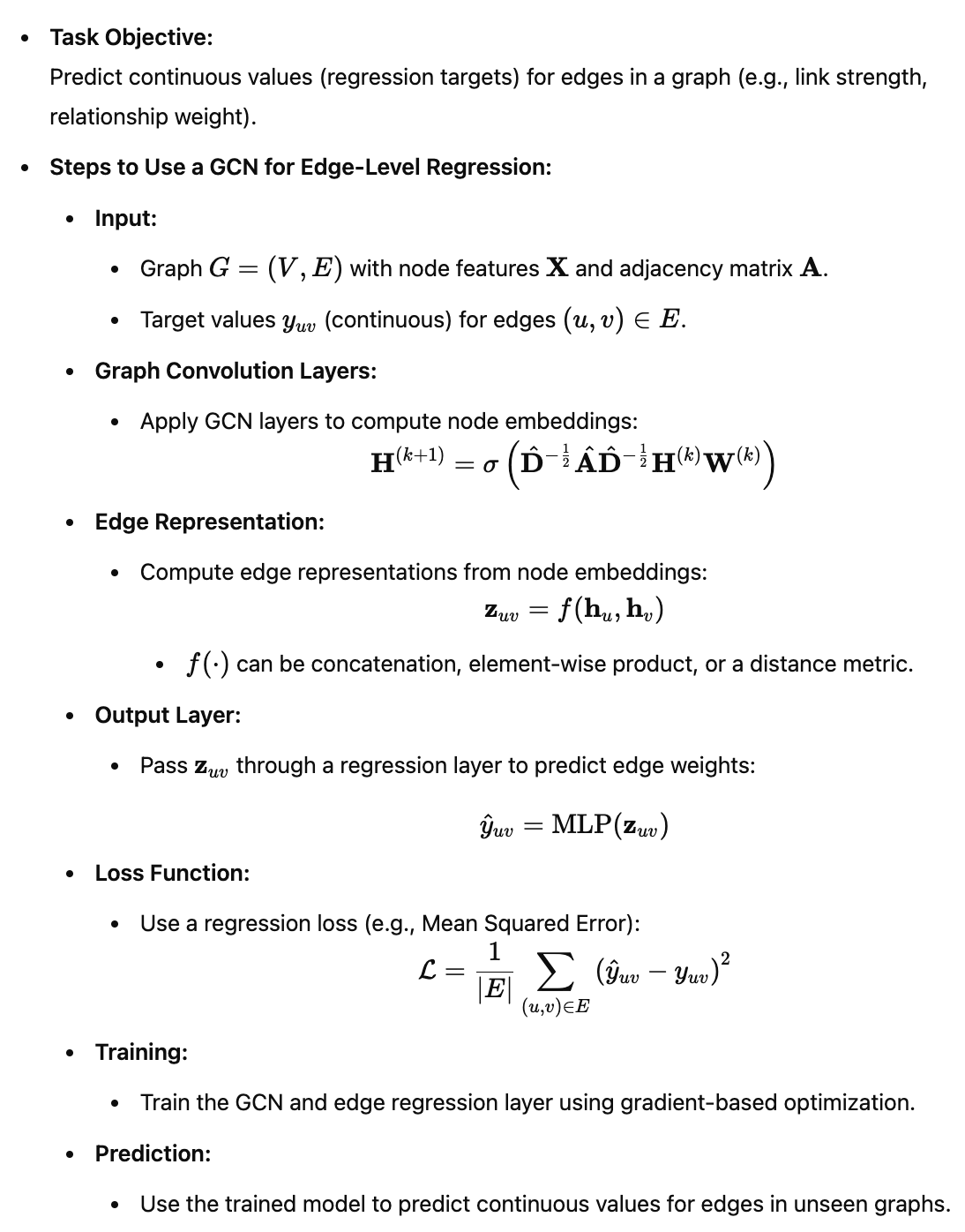
| Edge Classification | Combine embeddings of the two endpoint nodes | Edge class (exists, type, relationship) |
| Edge Regression | Combine embeddings of the two endpoint nodes | Continuous edge value (weight, distance, score) |
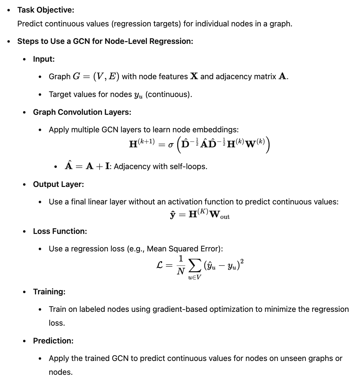
Node-Level Tasks
Node Embedding (hᵢ)
        │
        ▼
 Fully Connected Layer
        │
        ▼
 Prediction
Each node is processed independently after message passing.
Graph Pooling
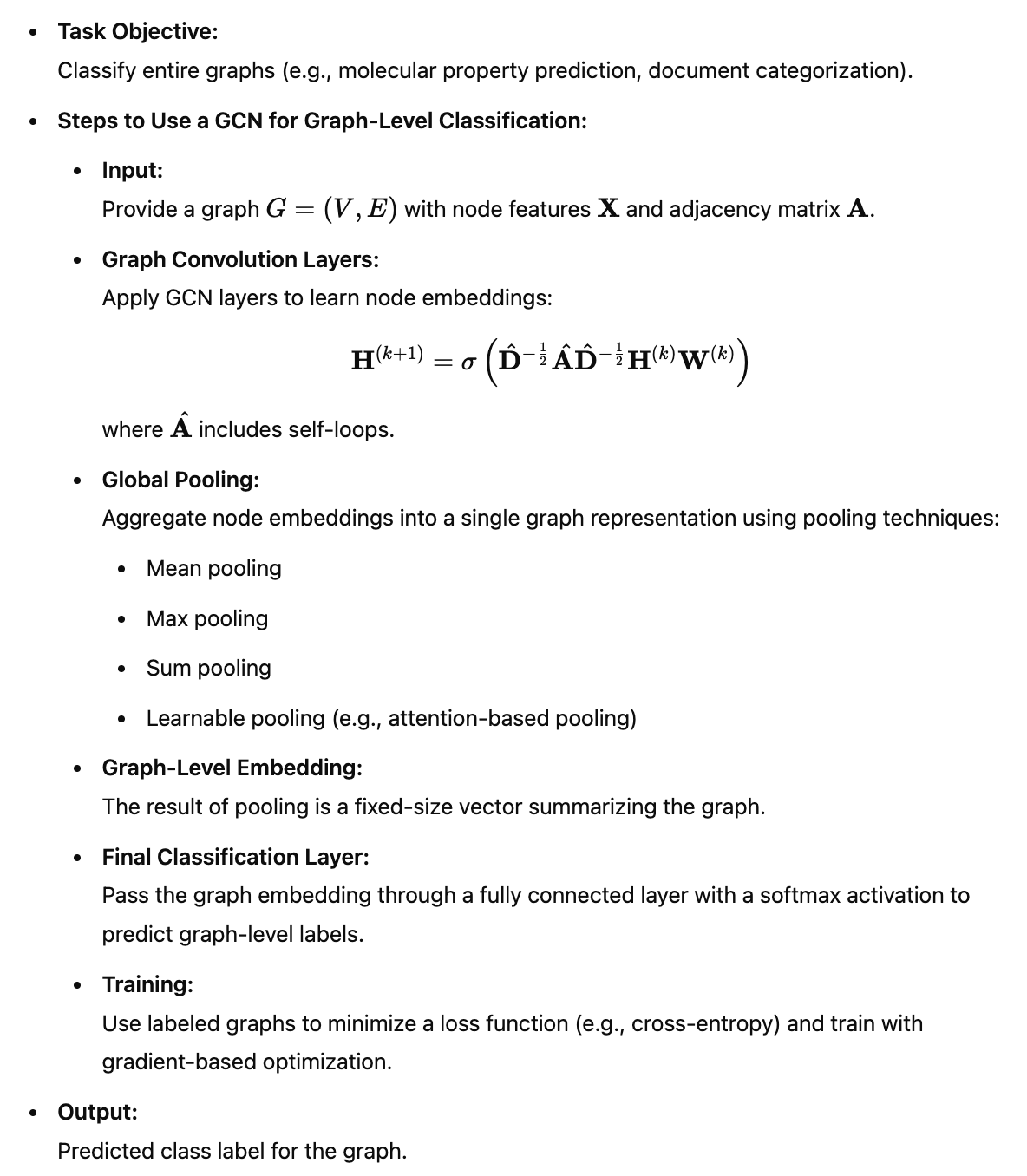
For graph-level prediction, the GCN produces an embedding for every node. Since graphs contain different numbers of nodes, these embeddings must be pooled into a single fixed-length graph embedding before making a prediction.
Common pooling methods include:
- Mean pooling: Average all node embeddings (most common and intuitive).
- Sum pooling: Add all node embeddings together (captures graph size).
- Max pooling: Take the maximum value of each embedding feature (captures the strongest signals).
- Attention pooling: Learn an importance weight for each node and compute a weighted average.
Node Embeddings
(h₁, h₂, ..., hₙ)
        │
        ▼
Global Pooling
(mean / sum / max / attention)
        │
        ▼
Graph Embedding
        │
        ▼
Prediction Head
The pooling operation is often called the graph readout layer because it converts a variable-sized set of node embeddings into a single graph representation suitable for graph classification or regression.
Graph-Level Tasks
All Node Embeddings
(h₁, h₂, ..., hₙ)
        │
        ▼
 Global Pooling
(mean / sum / max / attention)
        │
        ▼
 Graph Embedding
        │
        ▼
 Fully Connected Layer
        │
        ▼
 Prediction
The node embeddings are aggregated into a single graph representation before making a prediction.
Edge-Level Tasks
Node Embedding hᵢ      Node Embedding hⱼ
        │                     │
        └──── Combine ─────────┘
      (concat, dot product,
        element-wise product)
               │
               ▼
      Fully Connected Layer
               │
               ▼
          Prediction
Predictions are made using the embeddings of the two nodes that define the edge.
Sources
This content is drawn primarily from the following sources:
- Machine Learning with PyTorch and Scikit-Learn: Develop Machine Learning and Deep Learning Models with Python Book by Liu Yuxi, Sebastian Raschka, and Vahid Mirjalili
- “A Gentle Introduction to Graph Neural Networks” https://distill.pub/2021/gnn-intro/
- “Graph neural network” https://en.wikipedia.org/wiki/Graph_neural_network
- Machine Learning with PyTorch and Scikit-Learn by Sebastian Raschka, Yuxi Liu, Vahid Mirjalili
- GPT-3.5 and GPT-4