Community Detection in Network Science
Introduction to Network Communities
Community Structure in Networks
- Community Structure: Refers to the organization of nodes in a network into groups.
- Dense Intra-group Connections: Nodes within the same group are highly interconnected.
- Sparse Inter-group Connections: Few connections exist between nodes of different groups.
- Significance: Helps in understanding the modular nature of networks, such as social, biological, or technological systems.
- Applications: Used in clustering, detecting functional modules, and understanding network dynamics.
- Challenges: Identifying communities accurately, especially in large and complex networks.
Example: Visual Community detection
- Sometimes communities are very obvious. e.g. plot using a force-directed network layout algorithm and they can be identified visually
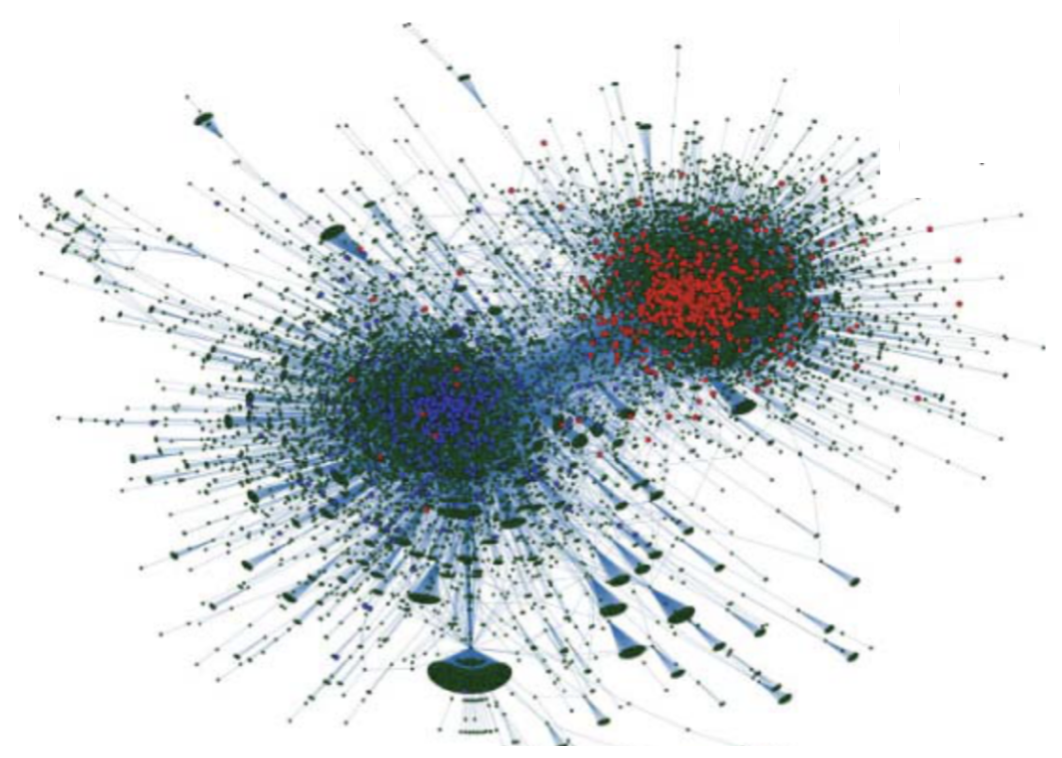
Retweet network of political hashtags prior to the 2010 US election.
- Node=User where liberal (blue) or conservative (red). , Link = retweet
Limitations of Visualization: In many small systems, visualization alone may not reveal clusters,
necessitating algorithmsthat can automatically detect them. ## Echo ChambersEcho Chambers and Filter Bubbles:
- These emerge when individuals are only exposed to others with similar ideas and beliefs.
- Understanding a network’s community structure can help classify nodes based on their positions within their clusters.
Real-World Network Communities
Social Networks: Groups of friends or followers on platforms like Facebook or Twitter, where members interact more frequently with each other than with outsiders.
Biological Networks: Functional groups of proteins in a cell that work together to perform specific biological processes.
Transportation Networks: Clusters of interconnected airports or train stations that facilitate regional travel more than long-distance connections.
Citation Networks: Academic papers that frequently cite each other, forming a community of related research topics.
Online Platforms: Subreddits or online forums where users with shared interests engage in discussions more often within the group than outside it.
Economic Networks: Companies within the same industry that trade more frequently with each other than with companies in other sectors.
Clustering vs. Community Detection
- Clustering:
- Groups similar nodes based on attributes or features.
- Often used in data mining and machine learning.
- Focuses on partitioning data into distinct groups.
- Examples: k-means, hierarchical clustering.
- Community Detection:
- Identifies groups of nodes with dense connections within a graph.
- Primarily used in network analysis.
- Emphasizes the structure and relationships in the network.
- Examples: modularity optimization, label propagation.
- Key Differences:
- Clustering is attribute-based; community detection is structure-based.
- Clustering can be applied to any data; community detection is specific to graphs.
- Applications:
- Clustering: market segmentation, image analysis.
- Community Detection: social network analysis, biological networks.
Community structure in networks
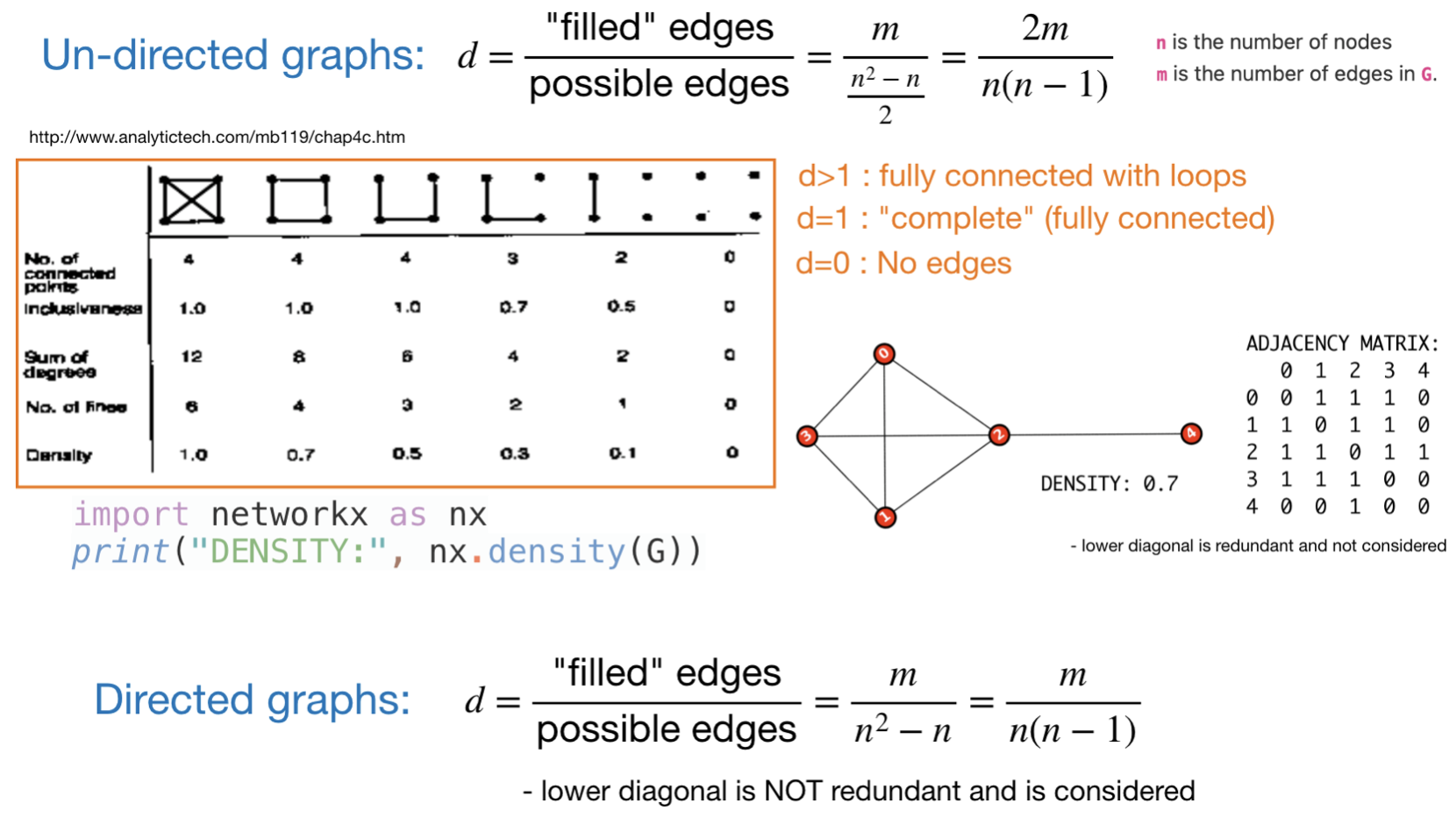
Recall: Global network Density
- Measure of graph’s connectivity
- property that quantifies the entire graph (not just a single node or edge)
- Fraction of “occupied edges” out of “total edges”
- also known as “wiring probability” or “connection probability”
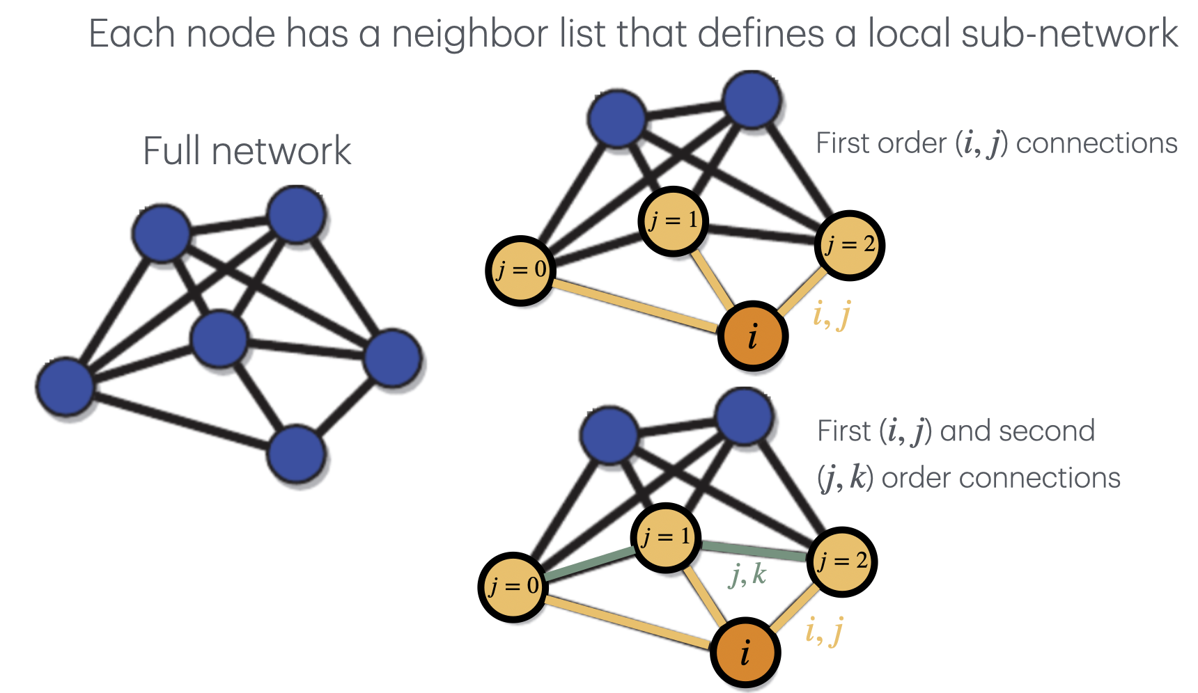
Neighbor list sub-networks
- Neighbor List Subnetwork: A subset of a larger network.
- Centered on Specific Node: Includes a node and its direct connections.
- Local Interactions: Captures interactions among immediate neighbors (local structure and dynamics).
Subgraphs and Components: Formally
- Subgraphs: A subgraph is a portion of a graph consisting of a subset of its vertices and edges.
- Example: Given a graph \(G = (V, E)\), a subgraph \(G' = (V', E')\) where \(V' \subseteq V\) and \(E' \subseteq E\).
- Connected Components: A connected component is a maximal subgraph where any two vertices are connected by a path.
- Example: In a graph with vertices \(\{A, B, C, D\}\) and edges \(\{(A, B), (B, C)\}\), \(\{A, B, C\}\) forms a connected component.
- Community Assignments: Communities are groups of vertices with dense connections internally and sparser connections externally.
- Example: In social networks, communities might represent groups of friends or colleagues.
- Visual Example:
- Graph: \(G = \{(A, B), (B, C), (D, E)\}\)
- Subgraph: \(G' = \{(A, B)\}\)
- Connected Components: \(\{\{A, B, C\}, \{D, E\}\}\)
Local density
- local density refers to the density of connections within a specific part of a network, typically a subgraph or a neighborhood around a particular node. Here’s a breakdown of what it involves:
- Connection Concentration: Local density measures the proportion of actual connections to the maximum possible connections within a defined area of the network.
- Neighborhood Focus: It often focuses on the immediate neighbors of a specific node, assessing how interconnected these neighbors are to each other.
- Indicative of Cohesiveness: Higher local densities suggest a tighter, more cohesive group of nodes, which may indicate a community or a clique within the network.
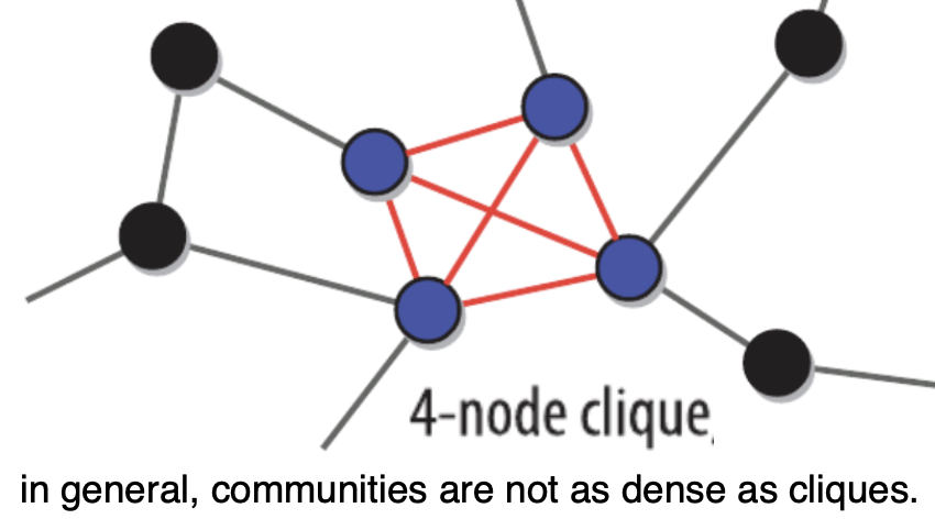
Clique
- Complete Subgraph: A clique is a subset of nodes within a graph where every pair of nodes is connected by an edge.
Region of Maximal local density- Maximal Connectivity: All nodes within the clique are directly linked to every other node in that group, indicating maximal inter-connectivity.
- Maximal Complete Subgraph: It represents the largest possible complete subgraph within a larger network where each node connects to every other node.
Communities
Communitiy overview
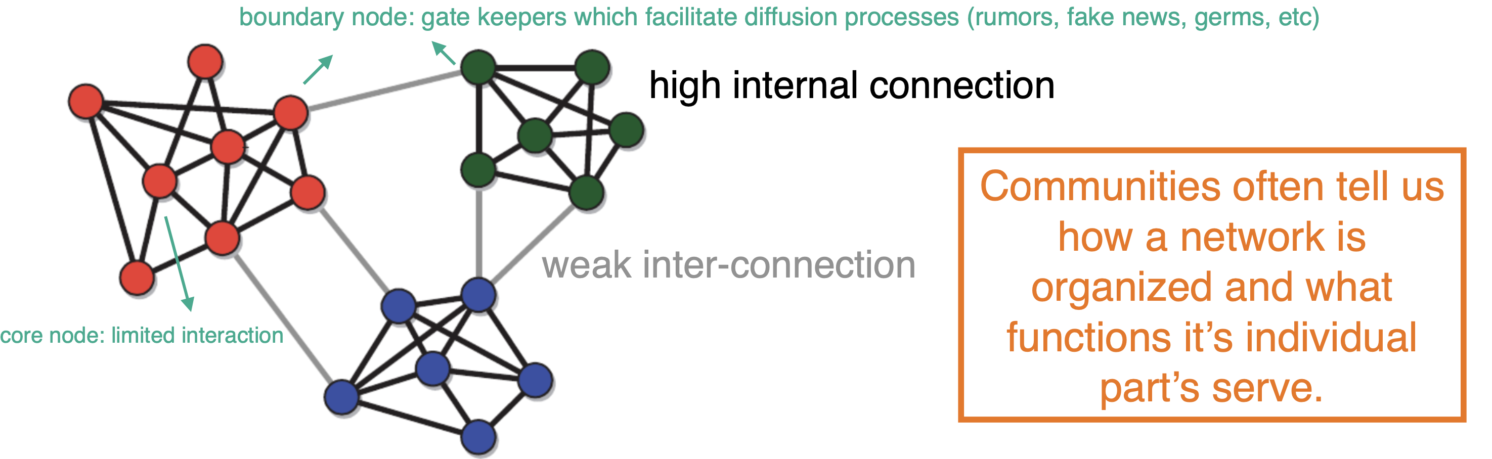
- Communities (i.e. modules or clusters)
- Sets of nodes with a
relatively higher connection densitywithin the cluster than between the clusters High intra-clusterlink density,lower inter-clusterlink density
- Sets of nodes with a
Cohesion and separation
Classic definitions of community-like structures are based on cohesion and on the interplay of cohesion and separation.
Community “definitions”
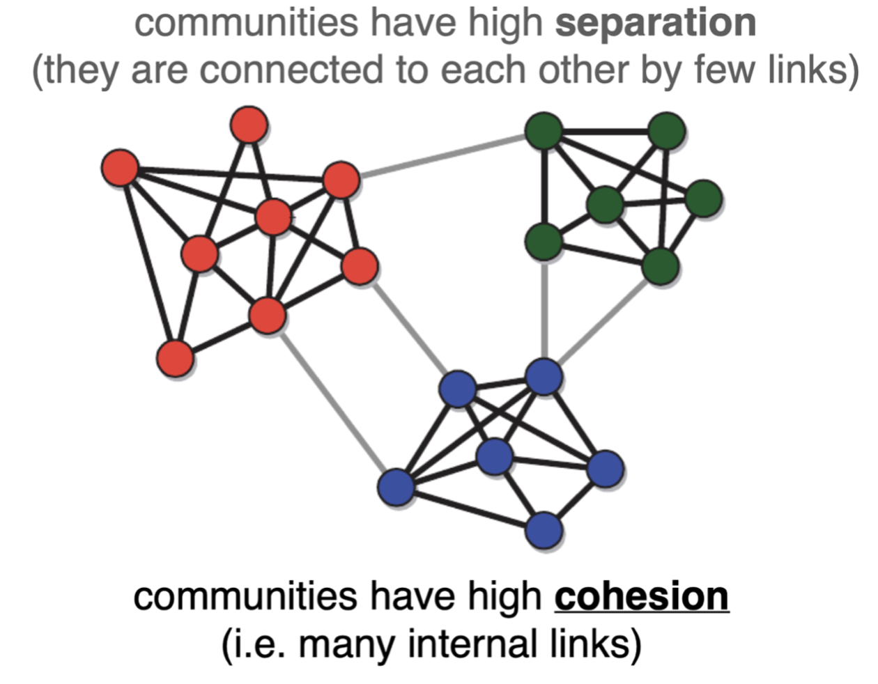
There is no unique definitionof a network community but the following is commonly adopted:- The link density within communities should be higher than the overall network density
- The link density across communities should be lower than the overall network density
Popular community definition: A sub-network where number of internal links is larger than the number of external links

Strong and weak Communities
strong community: Is a sub-network such that each node has more neighbors in the sub-network than in the rest of the network (internal degree > external degree)Weak community:A sub-network such that the sum of the internal degrees of all nodes exceeds the sum of their external degrees.
Overlapping Communities
- Definition: Overlapping communities occur when individuals belong to multiple groups simultaneously.
- Real-World Examples:
- Social networks: People often belong to various social circles (e.g., family, friends, colleagues).
- Professional affiliations: Individuals may be part of different professional organizations or teams.
- Relevance:
- Reflects complex social structures and interactions.
- Helps in understanding dynamics in social networks, marketing, and organizational behavior.
- Implications:
- Influences information spread and innovation diffusion.
- Affects group dynamics and decision-making processes.
- Challenges:
- Identifying and analyzing overlapping communities can be computationally complex.
- Requires sophisticated algorithms and models for accurate representation.
Partitions
Partitions: Introduction
Partition’sare particular division of a network into communities whereeach node belongs to only ONE community.
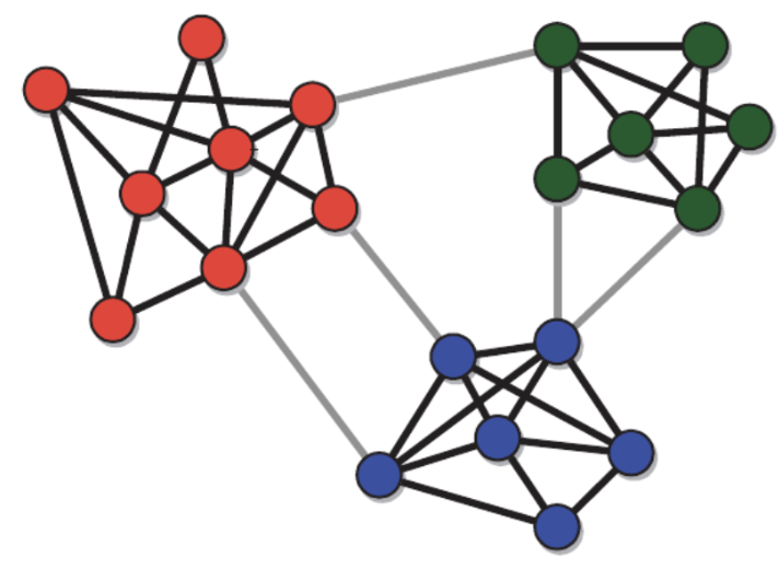
Common Properties- Partitions of real networks are often heterogeneous, i.e community properties may vary widely from one cluster to another.
- The cohesiveness is also highly variable, e.g. Internal community link density often spans several orders of magnitude, implying that some clusters are much more cohesive than others
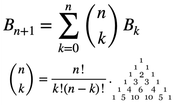
Bell number
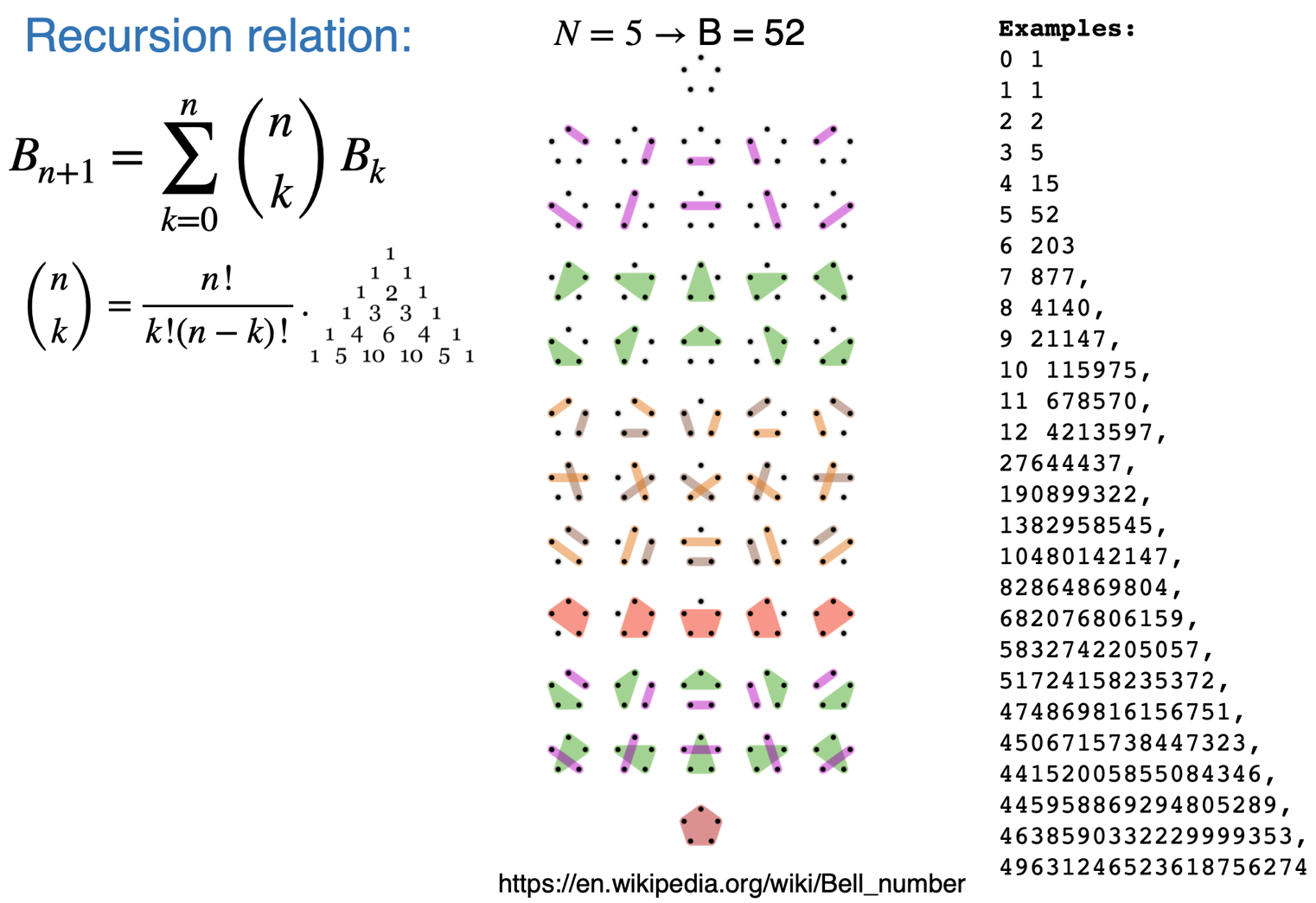
- Bell number (B) =
number of possible partitionsfor a given set of nodes N- Increases very fast with increased N (e.g. N = 12 B = 4213597)
- Makes it hard to algorithmically search for optimal partitions (can’t search all of them … there are just too many)
- Community detection algorithms typically explore only a tiny portion of the space of all partitions, where interesting solutions are most likely to be found.
Example: Recursion calculation
The triangular array whose right-hand diagonal sequence consists of Bell numbers

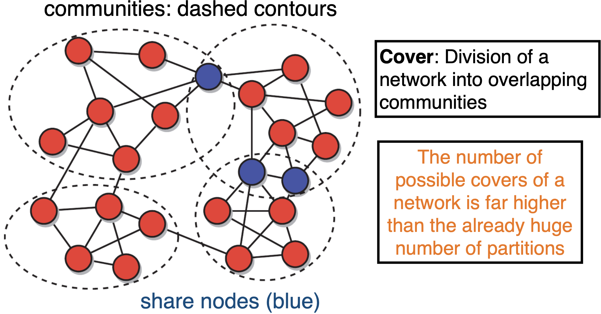
Overlapping communities:
- In
realitycommunities overlap (i.e. they share some of their nodes)(family, friends, work colleagues, etc) Cover:Division of a network into overlapping communities
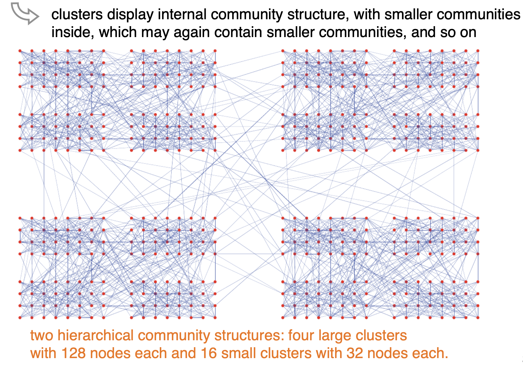
Hierarchical partitions
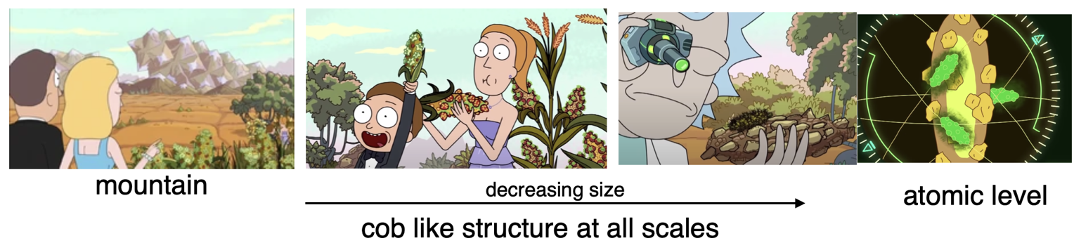
- Partitions can be hierarchical when the network has multiple levels of organization at different scales
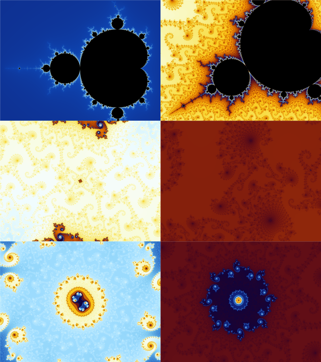
Aside: Fractals
- Hierarchical partitions are similar in some sense to Fractals
- Fractals are infinitely complex patterns that are self-similar across different scales.
- They are created by repeating a simple process over and over in an ongoing feedback loop.
- Driven by recursion, fractals are images of dynamic systems
Example-1:
Example-2:
Modularity
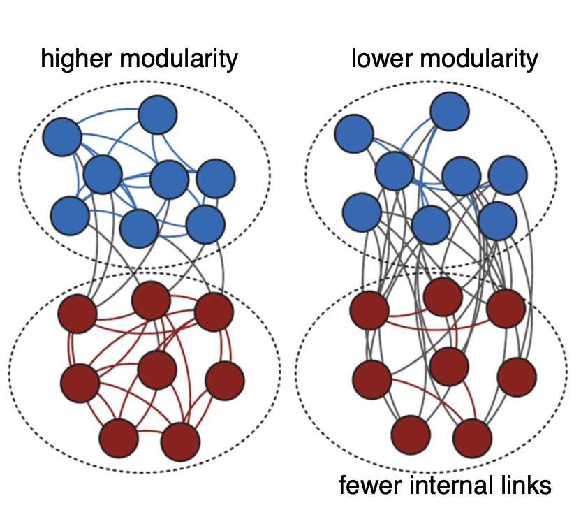
An important metric for evaluating the quality of a community detection algorithm.
Internal and external degree
Assume that we have defined a particular partition of the network into communities.
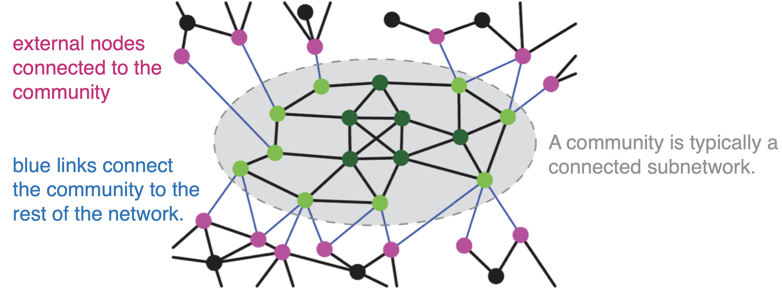
- A node’s
internal degreethe number of neighborsinsidethe community (number of black links) - A node’s
external degreethe number of neighborsoutsidethe community (number of blue links) - The
community degreeis the sum of the degrees of the nodes in the community; - The
internal link densityis the ratio between the number of internal links and the maximum number of links that could exist between any two community nodes. (i.e. Isolate internal sub-network and compute density as usual)
Modularity in Network Partitioning
- Definition: Modularity measures the strength of division of a network into modules (or communities).
- Purpose: Evaluates the quality of a network partition by comparing the density of links inside communities to links between communities.
- High Modularity: Indicates dense connections within communities and sparse connections between them.
- Range: Typically ranges from -1 to 1, where higher values suggest better-defined community structures.
- Applications: Used in social network analysis, biology, and computer science to identify community structures.
Modularity in Networks
- Modularity measures the strength of division of a network into modules (or communities).
- High modularity indicates dense connections within modules but sparse connections between them.
- Formula: \[ Q = \frac{1}{2m} \sum_{i,j} \left[ A_{ij} - \frac{k_i k_j}{2m} \right] \delta(c_i, c_j) \]
- \(A_{ij}\): adjacency matrix element (1 if edge exists, 0 otherwise)
- \(k_i, k_j\): degrees of nodes \(i\) and \(j\)
- \(m\): total number of edges
- \(\delta(c_i, c_j)\): 1 if nodes \(i\) and \(j\) are in the same community, 0 otherwise
- Interpretation:
- \(Q\) close to 1: strong community structure
- \(Q\) close to 0: no significant community structure
- Example: Consider a simple network with 4 nodes and 3 edges forming two communities. Calculate \(Q\) to evaluate community structure.
Modularity: Undirected case
- The modularity of a partition in an undirected, unweighted network is defined as
\[ Q=\frac{1}{L} \sum_C\left(L_C-\frac{k_C^2}{4 L}\right) \]
- where the sum runs over all clusters of the partition
- \(L_C\) is the number of internal links in cluster $C,
- k_C$ is the total degree of the nodes in \(C\),
- \(L\) is the number of links in the network.
- Partition of any network in a single cluster yields \(Q=0\)
Modularity can take negative values. e.g. A partition with \(N\) singletons:
Modularity: Directed case
- The expression of modularity for partitions of directed networks is
\[ Q_d=\frac{1}{L} \sum_C\left(L_C-\frac{k_C^{\text {in }} k_C^{o u t}}{L}\right), \]
- where \(L_C\) is the total number of directed links inside cluster \(C\)
- \(k_C^{\text {in }}, k_C^{\text {out }}\) are the total in-degree & out-degree of the nodes in \(C\), respectively.
Modularity
- The modularity of a partition evaluates the communities RELATIVE to a random baseline.
- Note: random networks do not have communities!

NetworkX: returns the modularity of the input partition
modularity = nx.community.quality.modularity(G, partition)
Maximum modularity
- When doing community detection we generally want partitions with
large modularity - For most networks, the modularity has a
non-trivial maximum: \(0<Q_{\max }<1\)
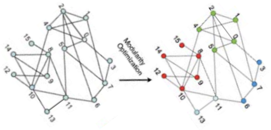
Modularity Optimization

- Starts from partition of singletons (negative modularity)
- Iteratively merges pairs of clusters which increase in modularity
- modularity increases steadily until a positive peak is reached,
- Eventually goes down until it hits zero when all nodes are in the same community.
- The partition corresponding to the peak value is the best solution found

Graph Bi-section
Graph Bi-section
Lets start simple with a binary partition
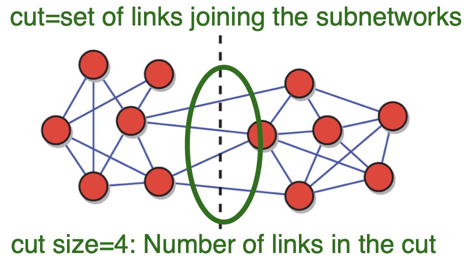
Graph bisection (minimum cut problem): binary partition case, network division into two clusters with equal number of nodes
- Definition: Splits graph vertices into two equal-sized sets while minimizing edge connections between them.
- Objective: To reduce the “cut size”—the number of edges linking the two subsets.
- Challenges: Optimizing bisection is NP-hard, complicating solutions for large graphs.
- Heuristic Methods: Employed due to complexity, including Kernighan–Lin, spectral partitioning, and multi-level partitioning.
- Evaluation Metrics: Assessed by cut size and the balance in subset sizes.
- Importance: Crucial for studying network structure and enhancing performance across applications.
Kernighan-Lin algorithm
- Popular network bisection algorithm
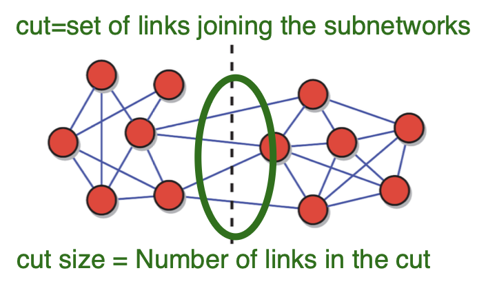
General idea:
- Start with an initial random network bisection (initial guess)
- swap pairs of nodes between the clusters to obtain the greatest decrease of the cut size, while the size of the clusters does not change
- repeat the process until no more swaps decrease cut size
Kernighan-Lin algorithm: closer look
Initial Partition: Begin with an arbitrary split of the network into two clusters \(A\) and \(B\), often by randomly dividing the nodes.
Iterative Refinement (Kernighan–Lin Algorithm):
- Step 1: For each \(i \in A\), \(j \in B\), calculate the change in cut size if \(i\) and \(j\) were swapped.
- Step 2: Identify the pair \((i^*, j^*)\) that produces the greatest cut size reduction; swap and lock them.
- Step 3: Repeat until no further swaps of unlocked nodes improve the cut size.
Termination Condition: The algorithm stops when successive iterations yield the same cut size—i.e., no further improvement is possible.
Generalization: The method can be extended beyond two clusters by considering node swaps between all cluster pairs.

Community Detection algorithms
Girvan-Newman algorithmLouvain methodLabel propagation
Community detection
Identifying communities in networks is an unsupervised task known by various terms, including community detection, community discovery, and clustering.
- Structure Identification: It reveals the modular structure within networks, highlighting densely connected clusters.
- Dynamics Insight: Understanding communities helps predict the spread of information or diseases.
- Functionality Analysis: It elucidates roles within networks, important in areas like biology.
- Algorithm Optimization: Community detection can improve tasks like data compression and network visualization.
- Targeted Interventions: Recognizing community structure aids in effective intervention in fields such as marketing or health.
- Enhanced Recommender Systems: Knowing community structures can refine recommendations by aligning with user group preferences.
- Anomaly Detection: Detects deviations from normal behaviors within network communities.
Network Partitioning
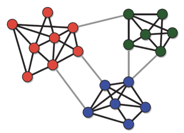
- Goal: Identifying well-separated sub-networks
- the focus is only on the
separationNOT cohesion, not always ideal for community defection - network partitioning search for balanced solutions
- the focus is only on the
- The partitioning problem consists
- finding a division of a network into a given number of sub-networks (or clusters), of given sizes,
- Subject to constraint that the total number of links connecting nodes in different sub-networks is minimized.
Comparision
Network Partitioning: A general graph division problem focused on splitting the graph into parts—often of similar size—while minimizing edge cuts between them. Typically used for load balancing in parallel computing.
Community Detection: Aims to uncover natural, densely connected groups of nodes with more internal edges than external ones. No constraint on group size; emphasizes structural cohesion, not balance.
Key Difference: Partitioning prioritizes balanced size and minimal cuts; community detection focuses on revealing meaningful modular structure.
Popular methods
- Louvain Method:
- Maximizes modularity score across the network.
- Efficient and effective for large networks.
- Girvan-Newman Algorithm: (bridge removal)
- Divisive method that removes edges based on betweenness centrality.
- Good for revealing smaller, more defined communities.
- Infomap:
- Uses random walks and information theory to detect communities.
- Minimizes the description length of random walks to define communities.
- Spectral Clustering:
- Utilizes eigenvectors of the network’s Laplacian matrix.
- Projects nodes into a lower-dimensional space for easier clustering.
- Label Propagation:
- Each node adopts the label most frequent among its neighbors.
- Fast and scalable, suitable for very large networks.
- Hierarchical Clustering:
- Builds a hierarchy of node clusters using either agglomerative or divisive approaches.
- Visualized using a dendrogram.
Hierarchical Clustering in Networks
Agglomerative vs Divisive Clustering
- Divisive Clustering:
- Starts with the entire network as a single cluster.
- Iteratively splits clusters into smaller ones.
- Often uses a top-down approach.
- Useful for identifying large, distinct clusters.
- Agglomerative Clustering:
- Begins with each node as its own cluster.
- Merges clusters iteratively based on similarity.
- Follows a bottom-up approach.
- Effective for discovering small, cohesive clusters.
- Comparison:
- Divisive is computationally intensive but can capture large-scale structures.
- Agglomerative is simpler and faster, suitable for detailed local structures.
- Choice depends on network size and desired granularity.
Scoring Mechanisms in Network Hierarchical Clustering (Concise)
Modularity: Measures how densely connected nodes are within communities vs. a random baseline; higher is better. Used to evaluate splits in divisive methods.
Edge Betweenness: Identifies edges likely connecting communities (high betweenness); guides removal in divisive algorithms like Girvan–Newman.
Linkage Criteria (Agglomerative): Merge clusters based on metrics like edge weights, average distances, or edge density.
Conductance / Normalized Cut: Measures how well a cluster is separated from the rest of the graph; lower values mean tighter clusters.
Stability: Assesses robustness of communities over perturbations or time; useful for choosing dendrogram levels.
Summary:
- Divisive methods use modularity, betweenness, and cut-based metrics.
- Agglomerative methods use network-adapted linkage scores.
Label Propagation Algorithm
Overview of Label Propagation
Purpose: Fast, scalable algorithm for community detection in large networks.
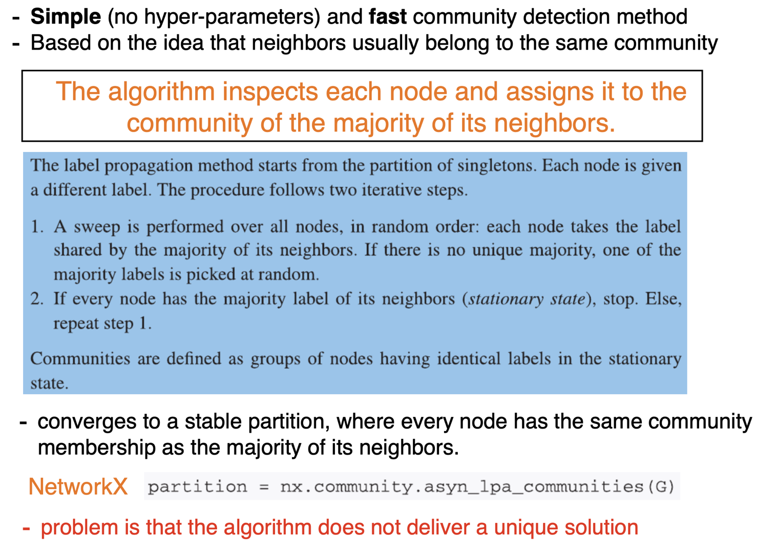
Key Idea: Nodes iteratively adopt the most frequent label among their neighbors.
Initialization:
- Each node is assigned a unique label.
Iteration Process:
- At each step, a node adopts the majority label in its neighborhood.
- Ties are broken randomly.
- Process repeats until labels converge.
Convergence:
- Algorithm stops when no label changes between iterations.
- Communities emerge as groups of nodes sharing the same label.
Advantages:
- No prior knowledge of the number of communities needed.
- Linear time complexity in the number of edges.
- Suitable for very large graphs.
Limitations:
- Non-deterministic results due to random tie-breaking.
- May produce unstable or trivial partitions.
Label Propagation: Closer look
Girvan-Newman algorithm
A Bridge removal algorithm
Recall: Node Between-ness centrality
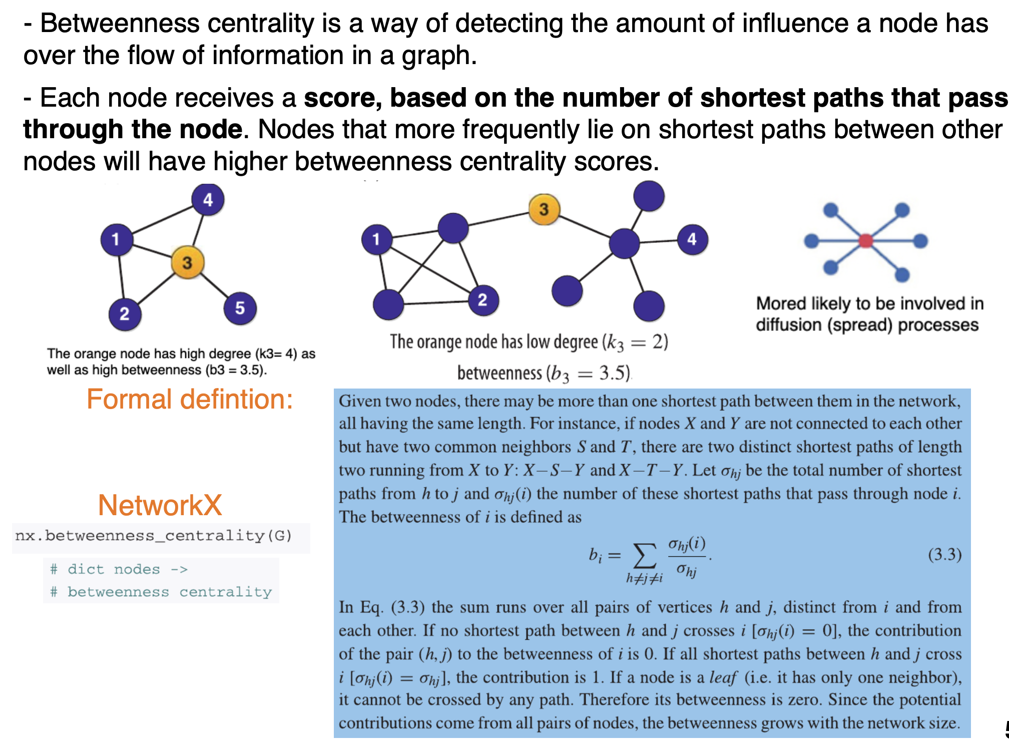
Edge betweenness
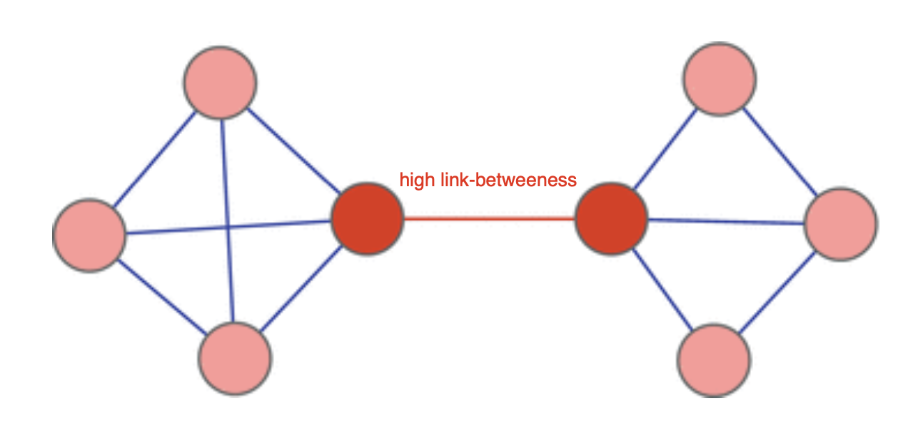
- The concept of node betweenness can be extended to links.
- The betweenness centrality of a link is the fraction of shortest paths among all possible node couples that pass through that link.
- Therefore link betweenness can be used to identify communities
- Links with very high betweenness centrality often join communities
- This Introduces an new link attribute (link betweenness)

Bridges
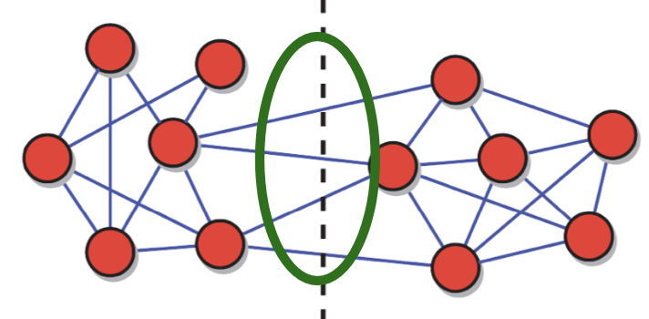
Strict definition:A bridge is a link whose removal breaks a connected network into two parts.Loose definition:Bridge is any link joining two communities

Overview of bridge removal
- Bridge Definition: An edge whose removal increases the number of connected components in a graph.
- Purpose in Community Detection: Bridge removal helps reveal densely connected communities by disconnecting weak inter-community links.
- Girvan–Newman Algorithm: Iteratively removes edges with highest betweenness centrality—often bridges—to expose community structure.
- Effect on Network: Increases network diameter, reduces connectivity, and may isolate nodes or subgraphs.
- Applications: Useful in analyzing social, biological, and communication networks to identify critical points of vulnerability or modular organization.
Bridge removal: Big picture
- Possible Community Detection method:
- Find bridges \(\rightarrow\) remove \(\rightarrow\) remaining GCC’s are the communities
Girvan-Newman algorithm
- The algorithm iteratively identifies and removes the links with largest edge-betweenness
- This leads to a progressive breakup of the network into disconnected pieces.
- Start by calculating the betweenness for all links.
- Then, each iteration of the algorithm consists of two steps:
- Remove the link with largest betweenness; in case of ties, one of them is picked at random.
- Recalculate the betweenness of the remaining links.
- The procedure ends when all links are removed and the nodes are isolated.

Louvain method
- Purpose: Detects communities in large networks.
- Approach: Greedy optimization of modularity.
- Modularity: Measures strength of division of a network into communities.
Louvain algorithm: Overview
The Louvain algorithm is a popular modularity optimization method
Purpose: The Louvain algorithm is designed for detecting communities in large networks efficiently.
Methodology: It uses a two-phase iterative optimization process:
- Phase 1: Each node is moved to the community that yields the highest gain in modularity.
- Phase 2: The algorithm aggregates nodes of the same community and builds a new network.
Repeat Process: These steps are repeated iteratively until modularity is maximized and cannot be increased further.
Performance: Known for its speed and scalability, making it suitable for very large networks. `* One benefit is that it is FAST!! can be used to detect communities in large networks with many millions of nodes and links.
Louvain algorithm: Closer look
- The algorithm starts again from the partition into singletons.
- Each iteration consists of two steps.
- Loop over the nodes: each node is put into the community of the neighbor that yields the largest modularity increase \(\Delta Q\) with respect to the current partition.
- All nodes are revisited over and over until it is no longer possible to increase \(Q\) by moving a node to a different community.
- The network is transformed into a weighted super-network, where each community in the partition from step 1 is replaced by a super-node, links between super-nodes carry a weight corresponding to the number of links joining nodes in the corresponding groups, and links joining nodes in the same community are represented as a self-loop from the corresponding super-node to itself, with weight equal to the number of internal links.
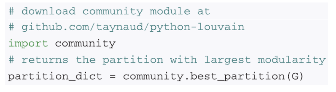
- Note: NetworkX does not yet have the Louvain algorithm, it requires and external library
Example: Simple Network
- Network: 4 nodes, edges between (1,2), (2,3), (3,4), (4,1).
- Initial Communities: \(\{1\}, \{2\}, \{3\}, \{4\}\).
- Optimization:
- Move node 1 to community of node 2 if gain is positive.
- Continue until no further gains.
- Output: Communities with maximum modularity.
Spectral Clustering
Spectral clustering can be used for multiple clusters—it is not limited to graph bisection.
Graph Bisection: Using the Fiedler vector (second-smallest eigenvector of the Laplacian) partitions the graph into two parts. This is the classic spectral bisection method.
Multiple Clusters (k-way clustering): Spectral clustering generalizes naturally:
- Compute the first \(k\) eigenvectors of the Laplacian (or normalized Laplacian).
- Treat each node as a point in a \(k\)-dimensional space (each coordinate from an eigenvector).
- Apply k-means (or another clustering algorithm) to group the nodes in this spectral space.
Why this works: The eigenvectors provide a low-dimensional embedding that preserves the graph’s community structure. Nodes in the same true cluster tend to be close together in this embedding.
Conclusion: Spectral clustering is a powerful, flexible method for detecting two or more clusters, especially in complex, non-convex, or graph-structured data.