Community Detection in Network Science

Introduction to Network Communities

Community Structure in Networks

  • Community Structure: Refers to the organization of nodes in a network into groups.
  • Dense Intra-group Connections: Nodes within the same group are highly interconnected.
  • Sparse Inter-group Connections: Few connections exist between nodes of different groups.
  • Significance: Helps in understanding the modular nature of networks, such as social, biological, or technological systems.
  • Applications: Used in clustering, detecting functional modules, and understanding network dynamics.
  • Challenges: Identifying communities accurately, especially in large and complex networks.

Example: Visual Community detection

  • Sometimes communities are very obvious. e.g. plot using a force-directed network layout algorithm and they can be identified visually
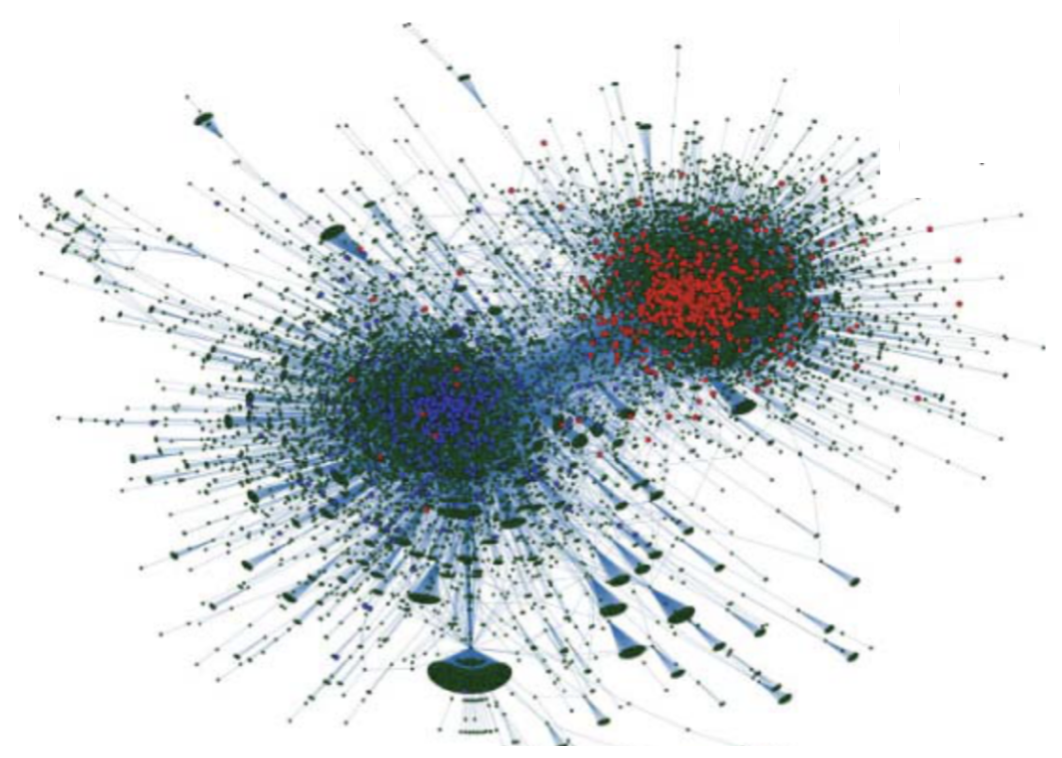
  • Retweet network of political hashtags prior to the 2010 US election.

    • Node=User where liberal (blue) or conservative (red). , Link = retweet
  • Limitations of Visualization: In many small systems, visualization alone may not reveal clusters, necessitating algorithms that can automatically detect them. ## Echo Chambers

  • Echo Chambers and Filter Bubbles:

    • These emerge when individuals are only exposed to others with similar ideas and beliefs.
    • Understanding a network’s community structure can help classify nodes based on their positions within their clusters.

Real-World Network Communities

  • Social Networks: Groups of friends or followers on platforms like Facebook or Twitter, where members interact more frequently with each other than with outsiders.

  • Biological Networks: Functional groups of proteins in a cell that work together to perform specific biological processes.

  • Transportation Networks: Clusters of interconnected airports or train stations that facilitate regional travel more than long-distance connections.

  • Citation Networks: Academic papers that frequently cite each other, forming a community of related research topics.

  • Online Platforms: Subreddits or online forums where users with shared interests engage in discussions more often within the group than outside it.

  • Economic Networks: Companies within the same industry that trade more frequently with each other than with companies in other sectors.

Clustering vs. Community Detection

  • Clustering:
    • Groups similar nodes based on attributes or features.
    • Often used in data mining and machine learning.
    • Focuses on partitioning data into distinct groups.
    • Examples: k-means, hierarchical clustering.
  • Community Detection:
    • Identifies groups of nodes with dense connections within a graph.
    • Primarily used in network analysis.
    • Emphasizes the structure and relationships in the network.
    • Examples: modularity optimization, label propagation.
  • Key Differences:
    • Clustering is attribute-based; community detection is structure-based.
    • Clustering can be applied to any data; community detection is specific to graphs.
  • Applications:
    • Clustering: market segmentation, image analysis.
    • Community Detection: social network analysis, biological networks.

Community structure in networks

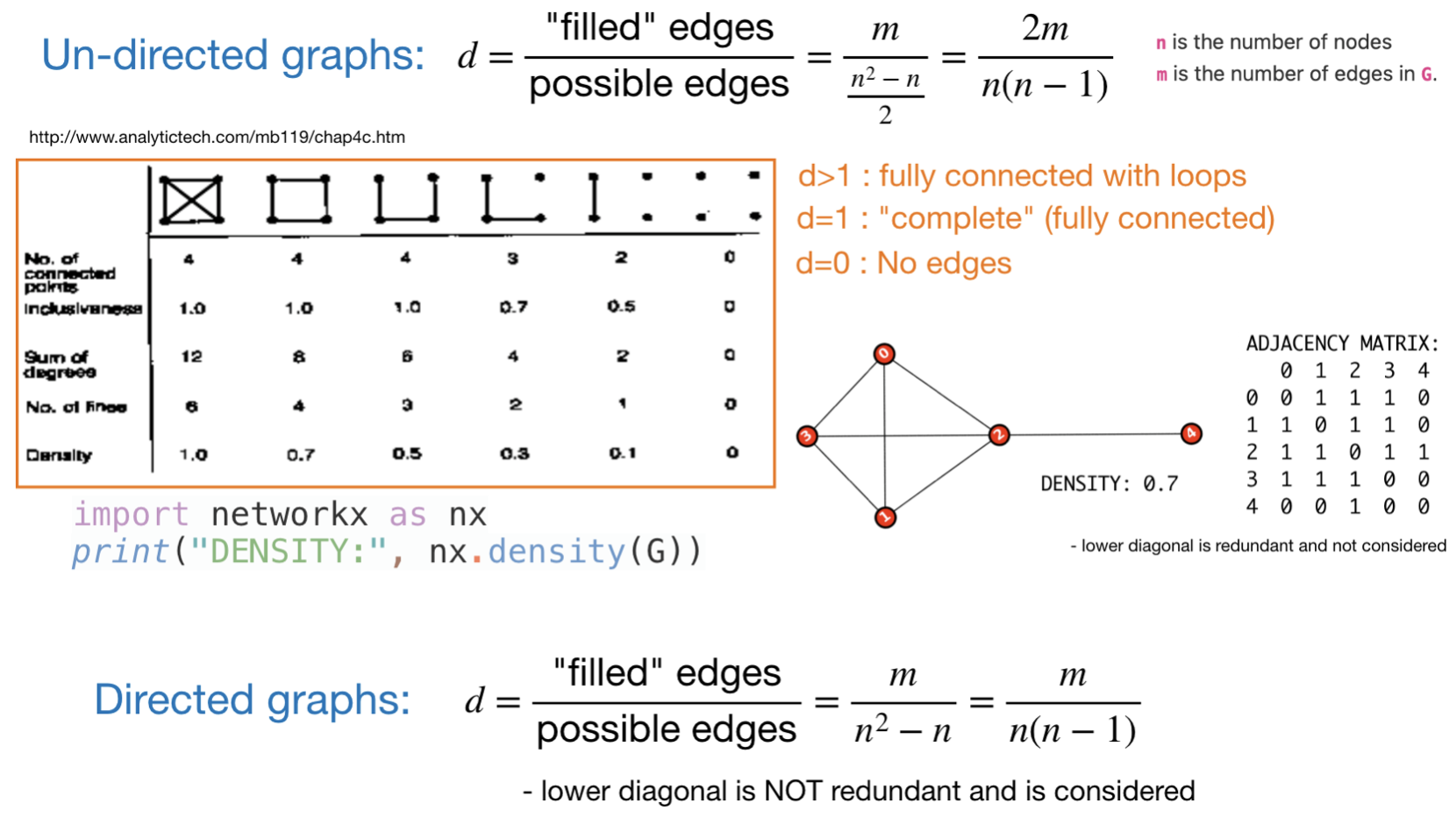
Recall: Global network Density

  • Measure of graph’s connectivity
    • property that quantifies the entire graph (not just a single node or edge)
    • Fraction of “occupied edges” out of “total edges”
    • also known as “wiring probability” or “connection probability”
Neighbor list sub-networks

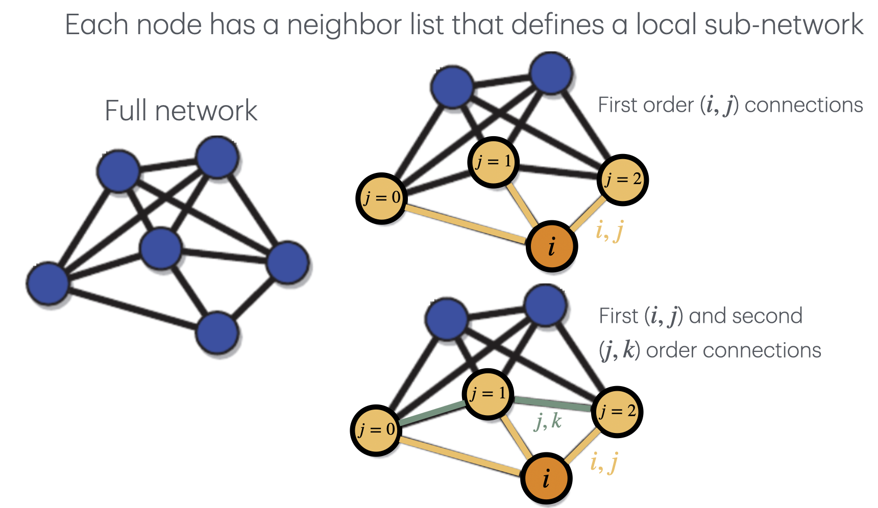
  • Neighbor List Subnetwork: A subset of a larger network.
  • Centered on Specific Node: Includes a node and its direct connections.
  • Local Interactions: Captures interactions among immediate neighbors (local structure and dynamics).
Subgraphs and Components: Formally

  • Subgraphs: A subgraph is a portion of a graph consisting of a subset of its vertices and edges.
    • Example: Given a graph \(G = (V, E)\), a subgraph \(G' = (V', E')\) where \(V' \subseteq V\) and \(E' \subseteq E\).
  • Connected Components: A connected component is a maximal subgraph where any two vertices are connected by a path.
    • Example: In a graph with vertices \(\{A, B, C, D\}\) and edges \(\{(A, B), (B, C)\}\), \(\{A, B, C\}\) forms a connected component.
  • Community Assignments: Communities are groups of vertices with dense connections internally and sparser connections externally.
    • Example: In social networks, communities might represent groups of friends or colleagues.
  • Visual Example:
    • Graph: \(G = \{(A, B), (B, C), (D, E)\}\)
    • Subgraph: \(G' = \{(A, B)\}\)
    • Connected Components: \(\{\{A, B, C\}, \{D, E\}\}\)

Local density

  • local density refers to the density of connections within a specific part of a network, typically a subgraph or a neighborhood around a particular node. Here’s a breakdown of what it involves:
    • Connection Concentration: Local density measures the proportion of actual connections to the maximum possible connections within a defined area of the network.
    • Neighborhood Focus: It often focuses on the immediate neighbors of a specific node, assessing how interconnected these neighbors are to each other.
    • Indicative of Cohesiveness: Higher local densities suggest a tighter, more cohesive group of nodes, which may indicate a community or a clique within the network.

Clique

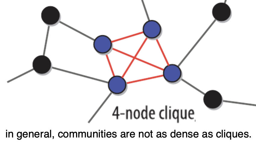
  • Complete Subgraph: A clique is a subset of nodes within a graph where every pair of nodes is connected by an edge.
  • Region of Maximal local density
  • Maximal Connectivity: All nodes within the clique are directly linked to every other node in that group, indicating maximal inter-connectivity.
  • Maximal Complete Subgraph: It represents the largest possible complete subgraph within a larger network where each node connects to every other node.
Communities

Communitiy overview

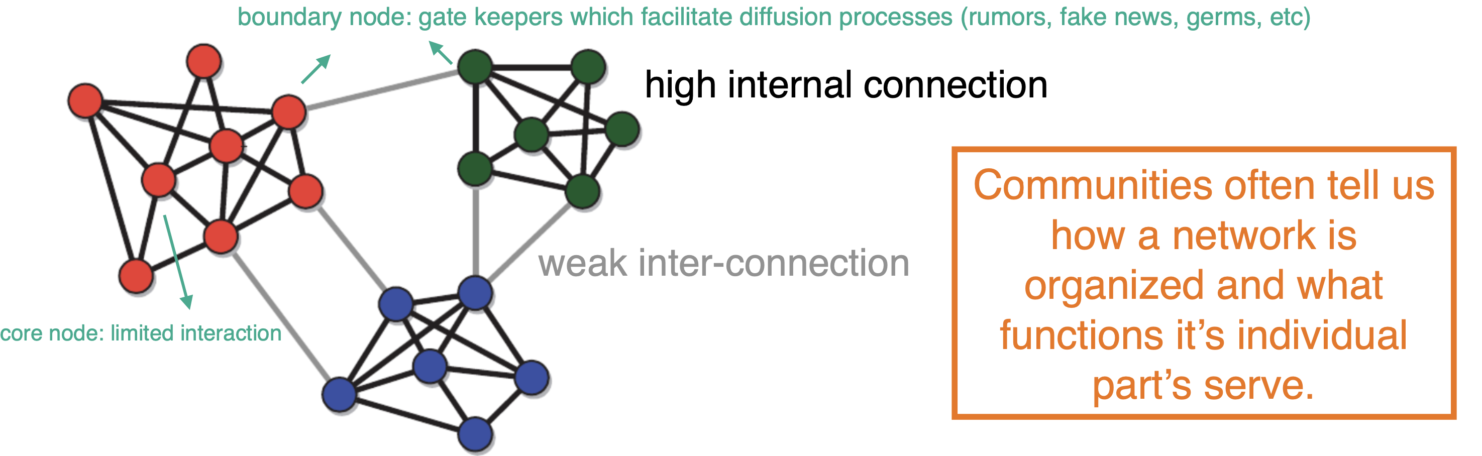
  • Communities (i.e. modules or clusters)
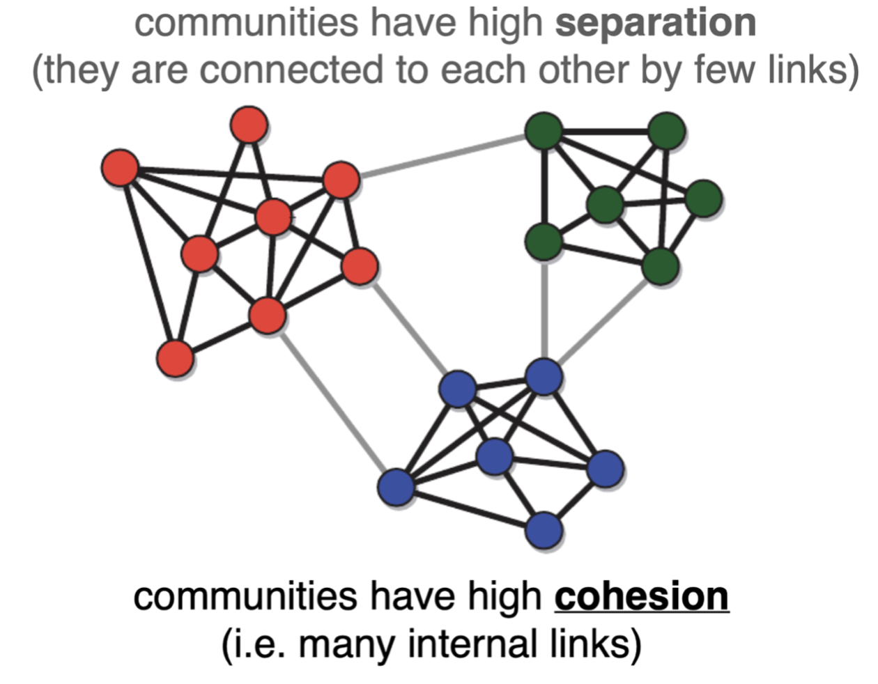
    • Sets of nodes with a relatively higher connection density within the cluster than between the clusters
    • High intra-cluster link density, lower inter-cluster link density

Cohesion and separation

Note

Classic definitions of community-like structures are based on cohesion and on the interplay of cohesion and separation.
Community “definitions”

  • There is no unique definition of a network community but the following is commonly adopted:
    • The link density within communities should be higher than the overall network density
    • The link density across communities should be lower than the overall network density

Popular community definition: A sub-network where number of internal links is larger than the number of external links

Strong and weak Communities

  • strong community: Is a sub-network such that each node has more neighbors in the sub-network than in the rest of the network (internal degree > external degree)
  • Weak community: A sub-network such that the sum of the internal degrees of all nodes exceeds the sum of their external degrees.

Overlapping Communities

  • Definition: Overlapping communities occur when individuals belong to multiple groups simultaneously.
  • Real-World Examples:
    • Social networks: People often belong to various social circles (e.g., family, friends, colleagues).
    • Professional affiliations: Individuals may be part of different professional organizations or teams.
  • Relevance:
    • Reflects complex social structures and interactions.
    • Helps in understanding dynamics in social networks, marketing, and organizational behavior.
  • Implications:
    • Influences information spread and innovation diffusion.
    • Affects group dynamics and decision-making processes.
  • Challenges:
    • Identifying and analyzing overlapping communities can be computationally complex.
    • Requires sophisticated algorithms and models for accurate representation.

Partitions

Partitions: Introduction

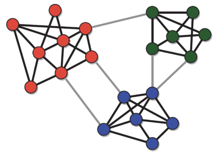
  • Partition’s are particular division of a network into communities where each node belongs to only ONE community.
  • Common Properties
    • Partitions of real networks are often heterogeneous, i.e community properties may vary widely from one cluster to another.
    • The cohesiveness is also highly variable, e.g. Internal community link density often spans several orders of magnitude, implying that some clusters are much more cohesive than others

Bell number

  • Bell number (B) = number of possible partitions for a given set of nodes N
    • Increases very fast with increased N (e.g. N = 12 B = 4213597)
    • Makes it hard to algorithmically search for optimal partitions (can’t search all of them … there are just too many)
  • Community detection algorithms typically explore only a tiny portion of the space of all partitions, where interesting solutions are most likely to be found.
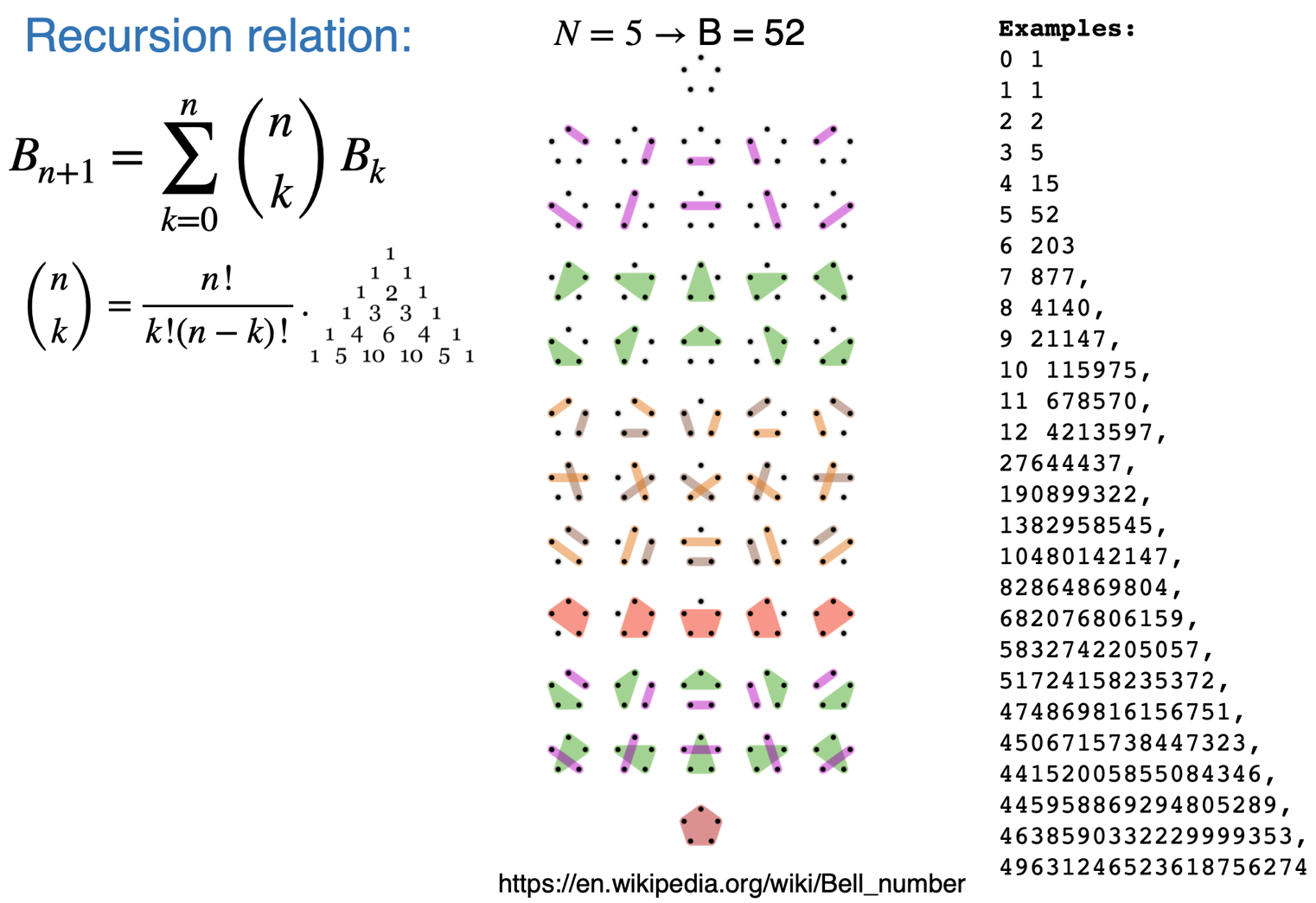
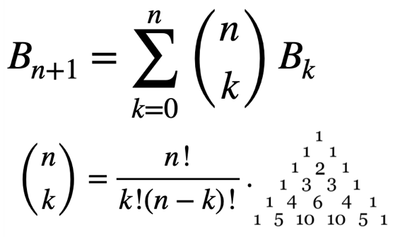
Example: Recursion calculation

The triangular array whose right-hand diagonal sequence consists of Bell numbers
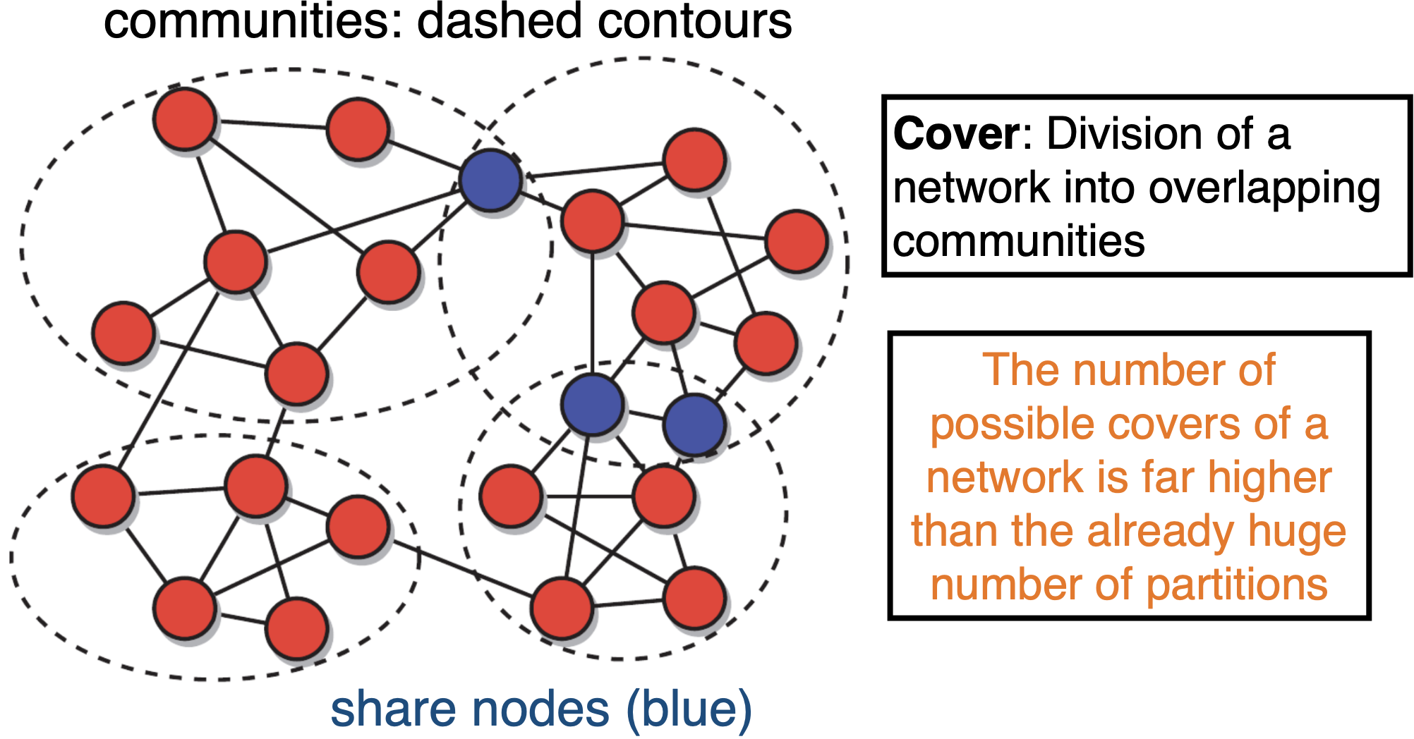
Overlapping communities:

  • In reality communities overlap (i.e. they share some of their nodes)(family, friends, work colleagues, etc)
  • Cover: Division of a network into overlapping communities
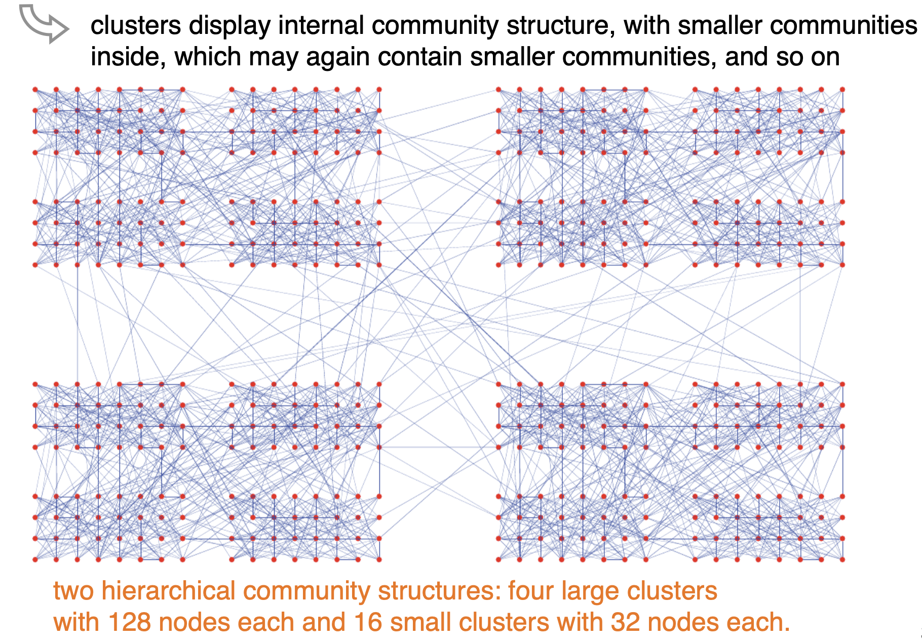
Hierarchical partitions

  • Partitions can be hierarchical when the network has multiple levels of organization at different scales
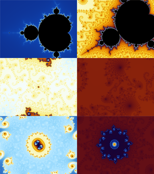
Aside: Fractals

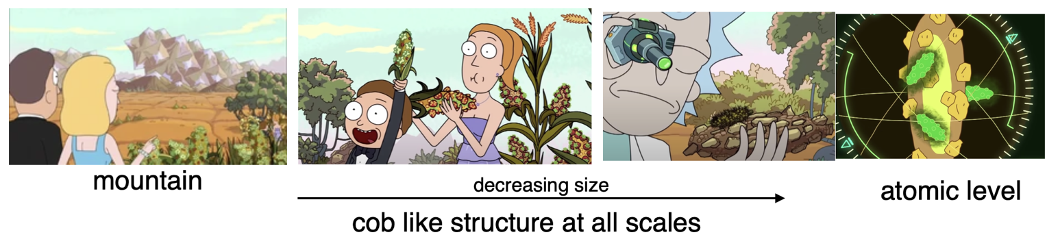
  • Hierarchical partitions are similar in some sense to Fractals
  • Fractals are infinitely complex patterns that are self-similar across different scales.
    • They are created by repeating a simple process over and over in an ongoing feedback loop.
    • Driven by recursion, fractals are images of dynamic systems

Example-1:
Example-2:
Modularity

An important metric for evaluating the quality of a community detection algorithm.

Internal and external degree

Assume that we have defined a particular partition of the network into communities.
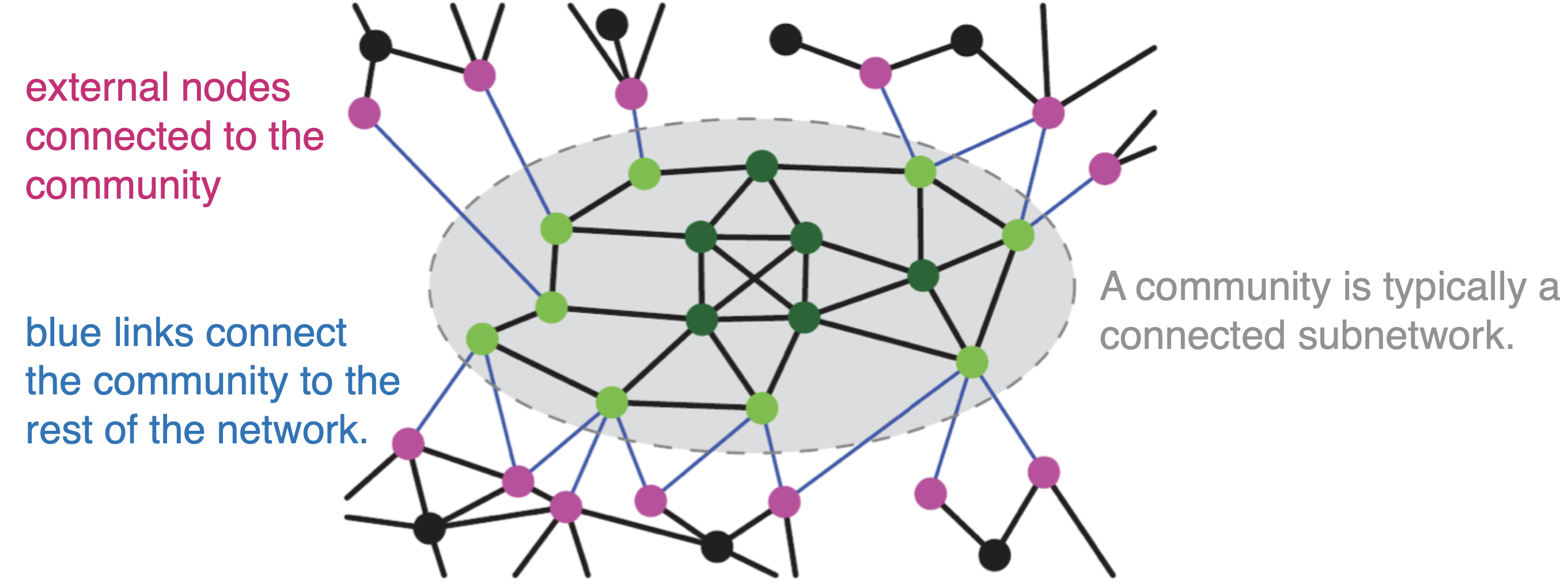
  • A node’s internal degree the number of neighbors inside the community (number of black links)
  • A node’s external degree the number of neighbors outside the community (number of blue links)
  • The community degree is the sum of the degrees of the nodes in the community;
  • The internal link density is the ratio between the number of internal links and the maximum number of links that could exist between any two community nodes. (i.e. Isolate internal sub-network and compute density as usual)

Modularity in Network Partitioning

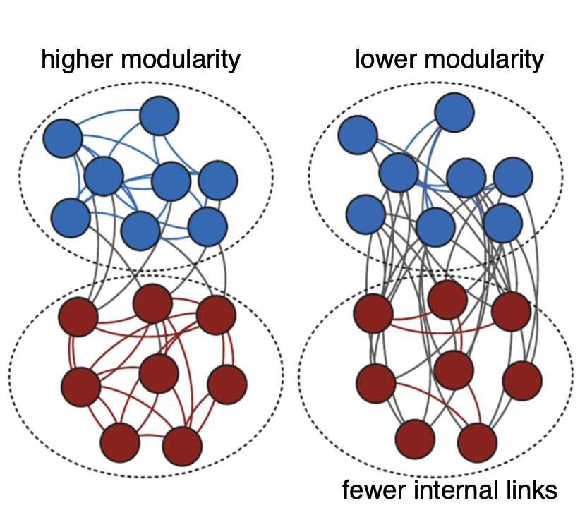
  • Definition: Modularity measures the strength of division of a network into modules (or communities).
  • Purpose: Evaluates the quality of a network partition by comparing the density of links inside communities to links between communities.
  • High Modularity: Indicates dense connections within communities and sparse connections between them.
  • Range: Typically ranges from -1 to 1, where higher values suggest better-defined community structures.
  • Applications: Used in social network analysis, biology, and computer science to identify community structures.

Modularity in Networks

  • Modularity measures the strength of division of a network into modules (or communities).
  • High modularity indicates dense connections within modules but sparse connections between them.
  • Formula: \[ Q = \frac{1}{2m} \sum_{i,j} \left[ A_{ij} - \frac{k_i k_j}{2m} \right] \delta(c_i, c_j) \]
    • \(A_{ij}\): adjacency matrix element (1 if edge exists, 0 otherwise)
    • \(k_i, k_j\): degrees of nodes \(i\) and \(j\)
    • \(m\): total number of edges
    • \(\delta(c_i, c_j)\): 1 if nodes \(i\) and \(j\) are in the same community, 0 otherwise
  • Interpretation:
    • \(Q\) close to 1: strong community structure
    • \(Q\) close to 0: no significant community structure
  • Example: Consider a simple network with 4 nodes and 3 edges forming two communities. Calculate \(Q\) to evaluate community structure.

Modularity: Undirected case

  • The modularity of a partition in an undirected, unweighted network is defined as

\[ Q=\frac{1}{L} \sum_C\left(L_C-\frac{k_C^2}{4 L}\right) \]

  • where the sum runs over all clusters of the partition
  • \(L_C\) is the number of internal links in cluster $C,
  • k_C$ is the total degree of the nodes in \(C\),
  • \(L\) is the number of links in the network.
  • Partition of any network in a single cluster yields \(Q=0\)
  • Modularity can take negative values. e.g. A partition with \(N\) singletons:

Modularity: Directed case

  • The expression of modularity for partitions of directed networks is

\[ Q_d=\frac{1}{L} \sum_C\left(L_C-\frac{k_C^{\text {in }} k_C^{o u t}}{L}\right), \]

  • where \(L_C\) is the total number of directed links inside cluster \(C\)
  • \(k_C^{\text {in }}, k_C^{\text {out }}\) are the total in-degree & out-degree of the nodes in \(C\), respectively.

Modularity

  • The modularity of a partition evaluates the communities RELATIVE to a random baseline.
    • Note: random networks do not have communities!

NetworkX: returns the modularity of the input partition

modularity = nx.community.quality.modularity(G, partition)

Maximum modularity

  • When doing community detection we generally want partitions with large modularity
  • For most networks, the modularity has a non-trivial maximum: \(0<Q_{\max }<1\)
Modularity Optimization

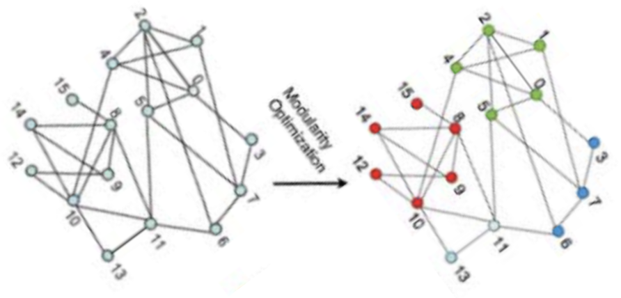
  • Starts from partition of singletons (negative modularity)
    • Iteratively merges pairs of clusters which increase in modularity
    • modularity increases steadily until a positive peak is reached,
    • Eventually goes down until it hits zero when all nodes are in the same community.
    • The partition corresponding to the peak value is the best solution found
Graph Bi-section

Graph Bi-section

Lets start simple with a binary partition

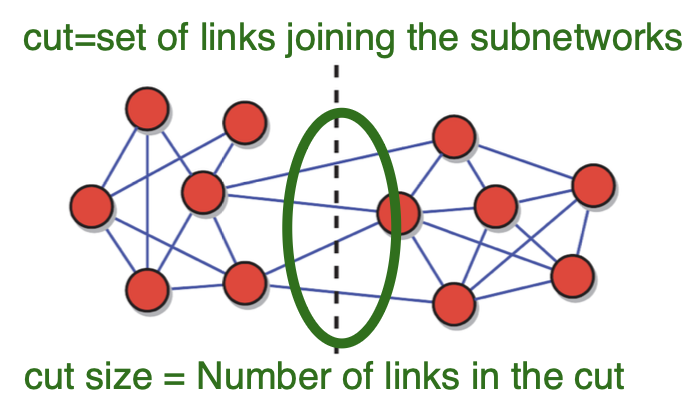
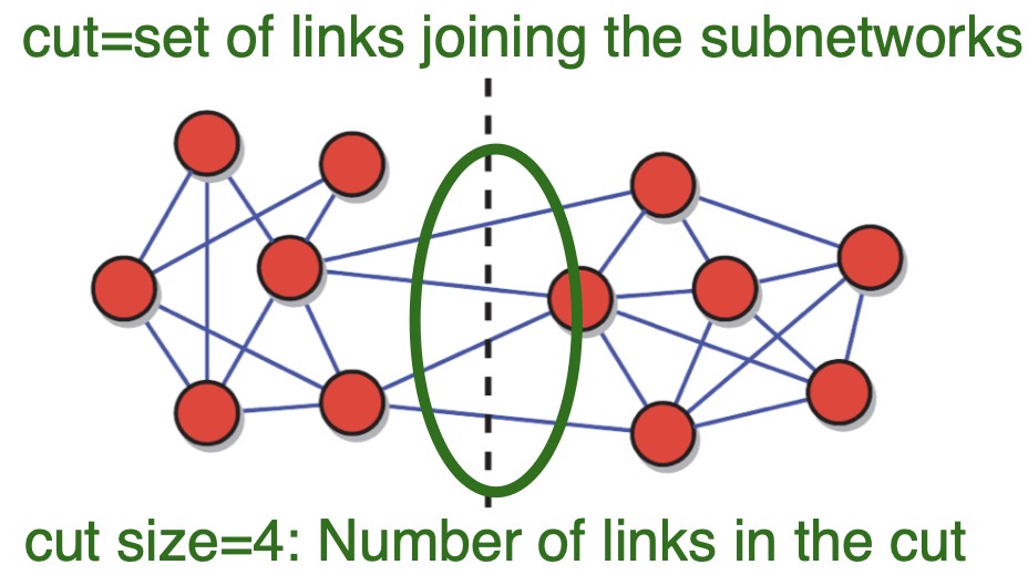
Graph bisection (minimum cut problem): binary partition case, network division into two clusters with equal number of nodes

  • Definition: Splits graph vertices into two equal-sized sets while minimizing edge connections between them.
  • Objective: To reduce the “cut size”—the number of edges linking the two subsets.
  • Challenges: Optimizing bisection is NP-hard, complicating solutions for large graphs.
  • Heuristic Methods: Employed due to complexity, including Kernighan–Lin, spectral partitioning, and multi-level partitioning.
  • Evaluation Metrics: Assessed by cut size and the balance in subset sizes.
  • Importance: Crucial for studying network structure and enhancing performance across applications.
Kernighan-Lin algorithm

  • Popular network bisection algorithm

General idea:

    1. Start with an initial random network bisection (initial guess)
    1. swap pairs of nodes between the clusters to obtain the greatest decrease of the cut size, while the size of the clusters does not change
    1. repeat the process until no more swaps decrease cut size

Kernighan-Lin algorithm: closer look

  • Initial Partition: Begin with an arbitrary split of the network into two clusters \(A\) and \(B\), often by randomly dividing the nodes.

  • Iterative Refinement (Kernighan–Lin Algorithm):

    • Step 1: For each \(i \in A\), \(j \in B\), calculate the change in cut size if \(i\) and \(j\) were swapped.
    • Step 2: Identify the pair \((i^*, j^*)\) that produces the greatest cut size reduction; swap and lock them.
    • Step 3: Repeat until no further swaps of unlocked nodes improve the cut size.
  • Termination Condition: The algorithm stops when successive iterations yield the same cut size—i.e., no further improvement is possible.

  • Generalization: The method can be extended beyond two clusters by considering node swaps between all cluster pairs.

Community Detection algorithms

  • Girvan-Newman algorithm
  • Louvain method
  • Label propagation

Community detection

Identifying communities in networks is an unsupervised task known by various terms, including community detection, community discovery, and clustering.

  • Structure Identification: It reveals the modular structure within networks, highlighting densely connected clusters.
  • Dynamics Insight: Understanding communities helps predict the spread of information or diseases.
  • Functionality Analysis: It elucidates roles within networks, important in areas like biology.
  • Algorithm Optimization: Community detection can improve tasks like data compression and network visualization.
  • Targeted Interventions: Recognizing community structure aids in effective intervention in fields such as marketing or health.
  • Enhanced Recommender Systems: Knowing community structures can refine recommendations by aligning with user group preferences.
  • Anomaly Detection: Detects deviations from normal behaviors within network communities.

Network Partitioning

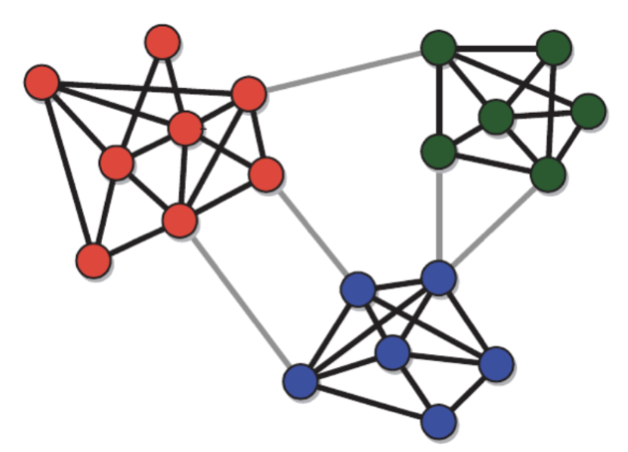
  • Goal: Identifying well-separated sub-networks
    • the focus is only on the separation NOT cohesion, not always ideal for community defection
    • network partitioning search for balanced solutions
  • The partitioning problem consists
      1. finding a division of a network into a given number of sub-networks (or clusters), of given sizes,
      1. Subject to constraint that the total number of links connecting nodes in different sub-networks is minimized.
Comparision

  • Network Partitioning: A general graph division problem focused on splitting the graph into parts—often of similar size—while minimizing edge cuts between them. Typically used for load balancing in parallel computing.

  • Community Detection: Aims to uncover natural, densely connected groups of nodes with more internal edges than external ones. No constraint on group size; emphasizes structural cohesion, not balance.

Key Difference: Partitioning prioritizes balanced size and minimal cuts; community detection focuses on revealing meaningful modular structure.

Hierarchical Clustering in Networks

Agglomerative vs Divisive Clustering

  • Divisive Clustering:
    • Starts with the entire network as a single cluster.
    • Iteratively splits clusters into smaller ones.
    • Often uses a top-down approach.
    • Useful for identifying large, distinct clusters.
  • Agglomerative Clustering:
    • Begins with each node as its own cluster.
    • Merges clusters iteratively based on similarity.
    • Follows a bottom-up approach.
    • Effective for discovering small, cohesive clusters.
  • Comparison:
    • Divisive is computationally intensive but can capture large-scale structures.
    • Agglomerative is simpler and faster, suitable for detailed local structures.
    • Choice depends on network size and desired granularity.

Scoring Mechanisms in Network Hierarchical Clustering (Concise)

  • Modularity: Measures how densely connected nodes are within communities vs. a random baseline; higher is better. Used to evaluate splits in divisive methods.

  • Edge Betweenness: Identifies edges likely connecting communities (high betweenness); guides removal in divisive algorithms like Girvan–Newman.

  • Linkage Criteria (Agglomerative): Merge clusters based on metrics like edge weights, average distances, or edge density.

  • Conductance / Normalized Cut: Measures how well a cluster is separated from the rest of the graph; lower values mean tighter clusters.

  • Stability: Assesses robustness of communities over perturbations or time; useful for choosing dendrogram levels.

Summary:

  • Divisive methods use modularity, betweenness, and cut-based metrics.
  • Agglomerative methods use network-adapted linkage scores.

Label Propagation Algorithm

Overview of Label Propagation

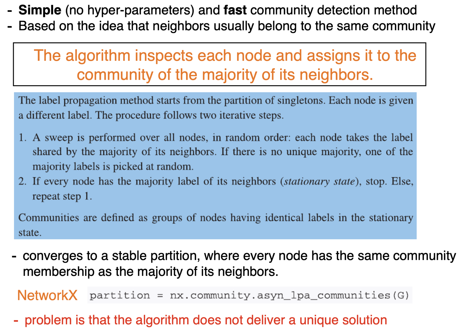
  • Purpose: Fast, scalable algorithm for community detection in large networks.

  • Key Idea: Nodes iteratively adopt the most frequent label among their neighbors.

  • Initialization:

    • Each node is assigned a unique label.
  • Iteration Process:

    • At each step, a node adopts the majority label in its neighborhood.
    • Ties are broken randomly.
    • Process repeats until labels converge.
  • Convergence:

    • Algorithm stops when no label changes between iterations.
    • Communities emerge as groups of nodes sharing the same label.
  • Advantages:

    • No prior knowledge of the number of communities needed.
    • Linear time complexity in the number of edges.
    • Suitable for very large graphs.
  • Limitations:

    • Non-deterministic results due to random tie-breaking.
    • May produce unstable or trivial partitions.

Label Propagation: Closer look

Girvan-Newman algorithm

A Bridge removal algorithm

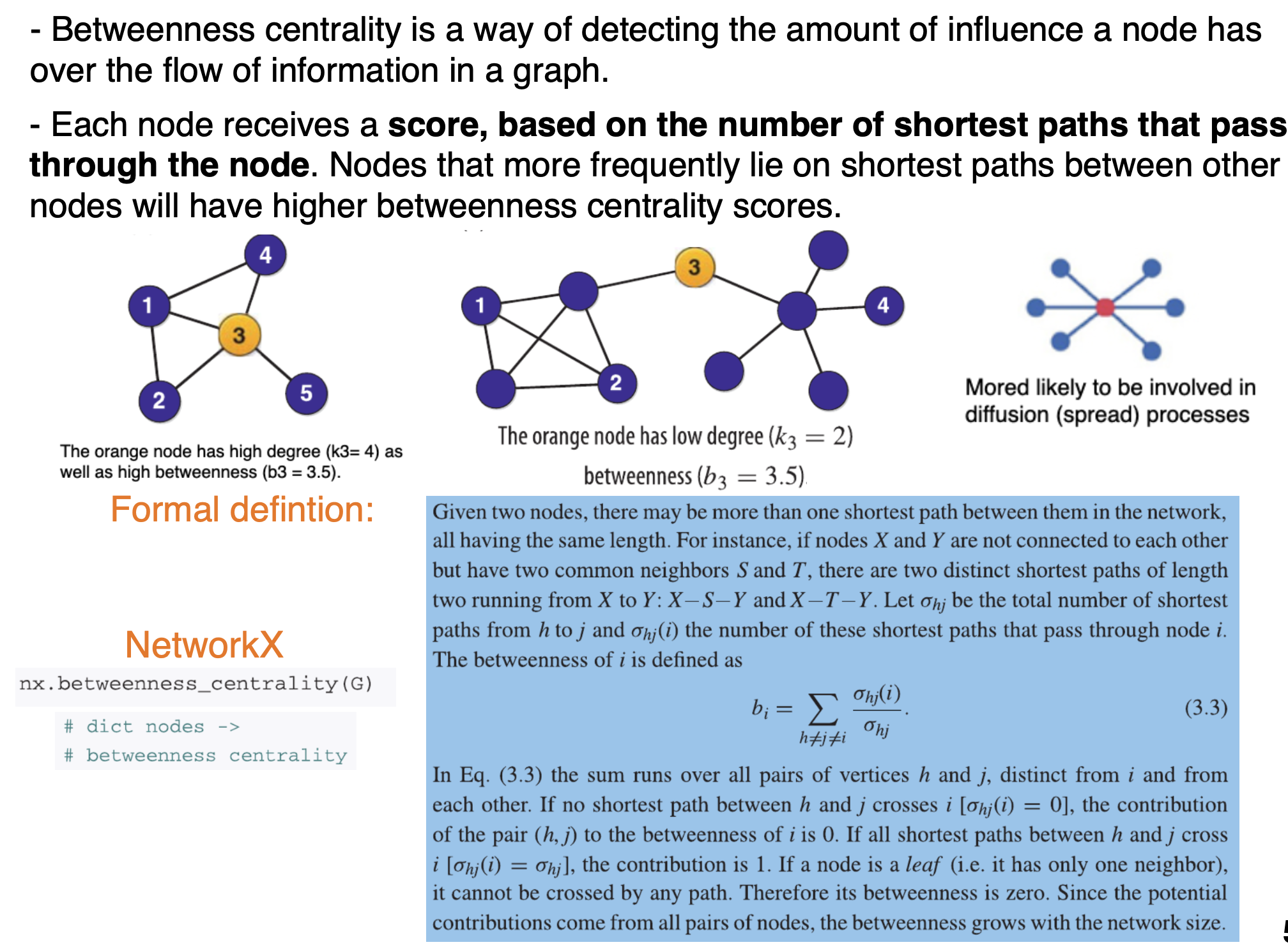
Recall: Node Between-ness centrality

Edge betweenness

  • The concept of node betweenness can be extended to links.
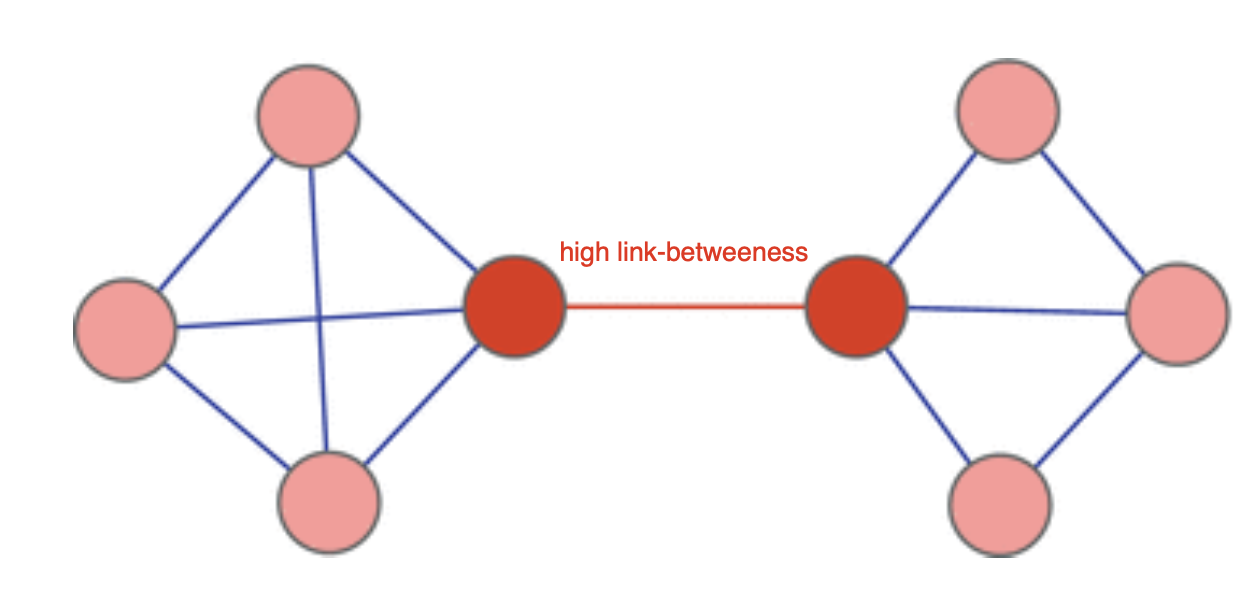
  • The betweenness centrality of a link is the fraction of shortest paths among all possible node couples that pass through that link.
  • Therefore link betweenness can be used to identify communities
  • Links with very high betweenness centrality often join communities
  • This Introduces an new link attribute (link betweenness)
Bridges

  • Strict definition: A bridge is a link whose removal breaks a connected network into two parts.
  • Loose definition: Bridge is any link joining two communities

Overview of bridge removal

  • Bridge Definition: An edge whose removal increases the number of connected components in a graph.
  • Purpose in Community Detection: Bridge removal helps reveal densely connected communities by disconnecting weak inter-community links.
  • Girvan–Newman Algorithm: Iteratively removes edges with highest betweenness centrality—often bridges—to expose community structure.
  • Effect on Network: Increases network diameter, reduces connectivity, and may isolate nodes or subgraphs.
  • Applications: Useful in analyzing social, biological, and communication networks to identify critical points of vulnerability or modular organization.

Bridge removal: Big picture

  • Possible Community Detection method:
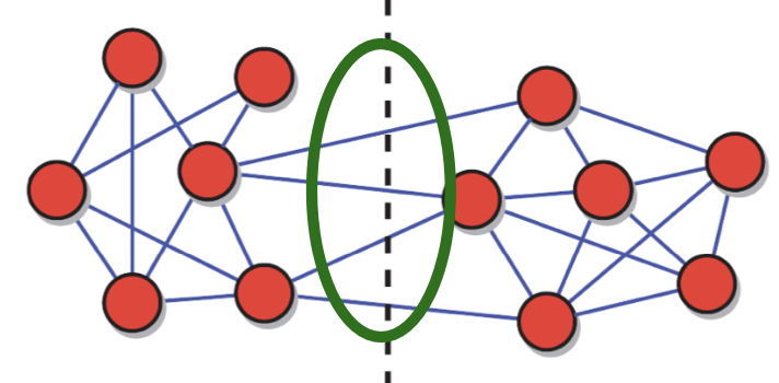
    • Find bridges \(\rightarrow\) remove \(\rightarrow\) remaining GCC’s are the communities
Girvan-Newman algorithm

  • The algorithm iteratively identifies and removes the links with largest edge-betweenness
  • This leads to a progressive breakup of the network into disconnected pieces.
  • Start by calculating the betweenness for all links.
  • Then, each iteration of the algorithm consists of two steps:
    1. Remove the link with largest betweenness; in case of ties, one of them is picked at random.
    2. Recalculate the betweenness of the remaining links.
  • The procedure ends when all links are removed and the nodes are isolated.

Louvain method

  • Purpose: Detects communities in large networks.
  • Approach: Greedy optimization of modularity.
  • Modularity: Measures strength of division of a network into communities.

Louvain algorithm: Overview

  • The Louvain algorithm is a popular modularity optimization method

  • Purpose: The Louvain algorithm is designed for detecting communities in large networks efficiently.

  • Methodology: It uses a two-phase iterative optimization process:

    • Phase 1: Each node is moved to the community that yields the highest gain in modularity.
    • Phase 2: The algorithm aggregates nodes of the same community and builds a new network.
  • Repeat Process: These steps are repeated iteratively until modularity is maximized and cannot be increased further.

  • Performance: Known for its speed and scalability, making it suitable for very large networks. `* One benefit is that it is FAST!! can be used to detect communities in large networks with many millions of nodes and links.

Louvain algorithm: Closer look

  • The algorithm starts again from the partition into singletons.
  • Each iteration consists of two steps.
      1. Loop over the nodes: each node is put into the community of the neighbor that yields the largest modularity increase \(\Delta Q\) with respect to the current partition.
      • All nodes are revisited over and over until it is no longer possible to increase \(Q\) by moving a node to a different community.
      1. The network is transformed into a weighted super-network, where each community in the partition from step 1 is replaced by a super-node, links between super-nodes carry a weight corresponding to the number of links joining nodes in the corresponding groups, and links joining nodes in the same community are represented as a self-loop from the corresponding super-node to itself, with weight equal to the number of internal links.
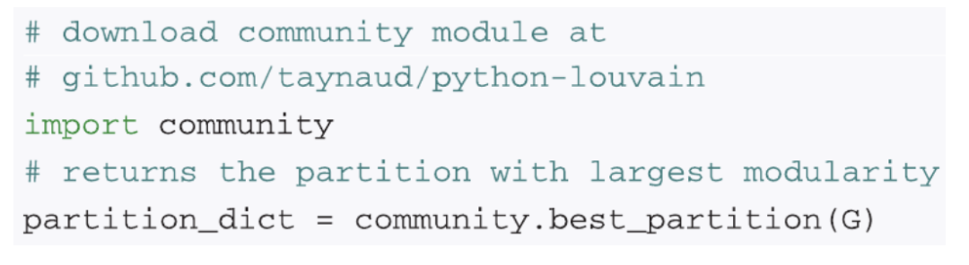
  • Note: NetworkX does not yet have the Louvain algorithm, it requires and external library
Example: Simple Network

  • Network: 4 nodes, edges between (1,2), (2,3), (3,4), (4,1).
  • Initial Communities: \(\{1\}, \{2\}, \{3\}, \{4\}\).
  • Optimization:
    • Move node 1 to community of node 2 if gain is positive.
    • Continue until no further gains.
  • Output: Communities with maximum modularity.

Spectral Clustering

Spectral clustering can be used for multiple clusters—it is not limited to graph bisection.

  • Graph Bisection: Using the Fiedler vector (second-smallest eigenvector of the Laplacian) partitions the graph into two parts. This is the classic spectral bisection method.

  • Multiple Clusters (k-way clustering): Spectral clustering generalizes naturally:

    1. Compute the first \(k\) eigenvectors of the Laplacian (or normalized Laplacian).
    2. Treat each node as a point in a \(k\)-dimensional space (each coordinate from an eigenvector).
    3. Apply k-means (or another clustering algorithm) to group the nodes in this spectral space.
  • Why this works: The eigenvectors provide a low-dimensional embedding that preserves the graph’s community structure. Nodes in the same true cluster tend to be close together in this embedding.

  • Conclusion: Spectral clustering is a powerful, flexible method for detecting two or more clusters, especially in complex, non-convex, or graph-structured data.