Breadth-first search algorithm
Overview
Important: Both BFS and DFS assume you have an adjacency list (or matrix) that tells you the neighbors of any node instantly.
Breadth-first search(BFS) is a core graph traversal method that explores a network from a source node, usually to find adesired attribute(often theshortest pathto every other node).- BFS explores all immediate neighbors before moving to their neighbors, creating a layered, “onion-like” search.
- It covers the entire “breadth” at each distance from the source before advancing to greater “depth.”
BFS explores all nodes at the current “level” (breadth) of the tree before going any deeper. It spreads outward like a ripple rather than diving down like DFS.
Applications
- Shortest path in unweighted graphs (BFS always finds the minimum number of hops between two nodes)
- Level-order tree traversal (visiting nodes layer by layer)
- Web crawlers (exploring links starting from a seed page, layer by layer outward)
- Social network distance (finding degrees of separation between people)
- Connected components (identifying which nodes can reach each other)
- Cycle detection in undirected graphs
- Bipartiteness testing (checking if a graph can be 2-colored with no conflicts)
- GPS/map routing (finding shortest routes on unweighted road networks)
Algorithm summary
- Initialization:
- Mark all nodes as unvisited.
- Create a queue and enqueue the source node, marking it as visited.
- Traversal:
- Dequeue a node from the queue and mark it as the current node.
- Process the current node (e.g., print its value or record its visitation).
- Enqueue all unvisited neighbors of the current node, marking them as visited.
- Repeat this process until the queue is empty.
Complexity
Time complexity: The algorithm visits every node and every edge just once, so the total amount of work is proportional to the number of nodes (\(V\)) plus the number of edges (\(E\)) in the graph. This is written as \(O(V + E)\), it’s efficient even on large graphs.
Space (memory)complexity: Breadth-first search keeps track of which nodes it needs to explore next (the queue) and which nodes it has already visited (the visited set). Both of these will use up to \(O(V)\) memory (RAM), meaning the amount of memory required is proportional to the number of nodes.
Breadth-First Search algorithm
- Breadth-first search (BFS) starts from a source node. Each node tracks its distance from the source.
- A queue;the “frontier”; manages nodes to visit, always processing the oldest node next (first-in, first-out).
- Begin by adding the source node \(s\) to the queue, set \(\ell(s, s) = 0\), and initialize all other nodes’ distances to -1. The shortest-path tree starts empty.
- At each step, dequeue the next node \(i\) from the frontier. For each unvisited neighbor \(j\) of \(i\):
- Enqueue \(j\).
- Set \(\ell_{s, j} = \ell_{s, i} + 1\) (distance from \(s\) to \(j\)).
- Add edge \((i \rightarrow j)\) to the shortest-path tree.
- The process repeats until the queue is empty. Nodes still marked with distance -1 are unreachable from the source and belong to other connected components.
Source: DOI:10.1017/97811086539471
Pseduo code for BFS
BFS(graph, start):
    queue ← [start]
    visited ← {start}

    while queue is not empty:
        node ← dequeue(queue)
        process(node)

        for each neighbor of node:
            if neighbor not in visited:
                visited.add(neighbor)
                enqueue(queue, neighbor)
Example
Consider the following undirected graph:
    A
   / \
  B   C
 / \   \
D E F- Start at node
A. - Enqueue
A, mark as visited. - Dequeue
A, process it. - Enqueue
BandC, mark them as visited. - Dequeue
B, process it. - Enqueue
DandE, mark them as visited. - Dequeue
C, process it. - Enqueue
F, mark it as visited. - Continue this process until the queue is empty.
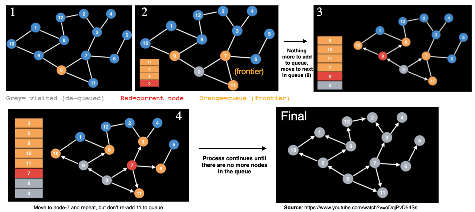
Example-1: Undirected case
- Imagine trying to find a particular node satisfying some criterion, or just the path length
- A logical method is to start with a random node, then check neighbors, then check neighbors of neighbors, and so on.
- We use a
queueto keep track of the process (For more details see: https://www.youtube.com/watch?v=oDqjPvD54Ss )
Example-2: Undirected case
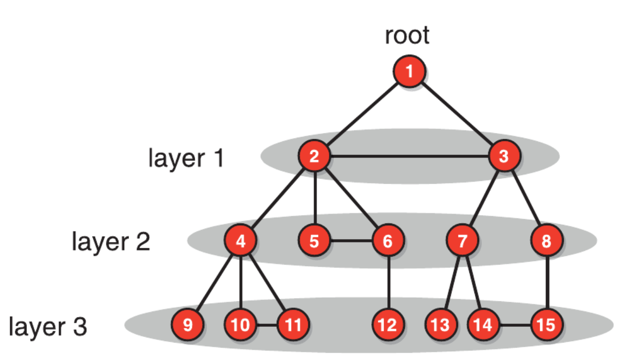
BFS naturally builds a tree by recording, for each node, which node discovered it (its “parent”), and because BFS processes nodes level by level, that parent relationship guarantees the path traced back from any node to the root through those parent pointers is the shortest possible path.
- Notice that the breadth-first search algorithm builds a directed
shortest-path tree - The tree maps the shortest paths between its root (the source node) and all other nodes.
- node-1 is selected as the source.
- visit the neighbors of node-1, which are 2 and 3. This is layer 1, including all nodes one step away from the source. We set the distance of those vertices from the source to one.
- Then we move to their neighbors 4,5,6,7,8, which are two steps away from the source (layer 2).
- Finally, we reach nodes 9,10,11,12,13,14,15, at distance three from the source (layer 3).
- Each layer contains all nodes having equal distance from the source.
- When completed, all nodes in the same connected component as the source have been assigned a distance from the source.
- To find the shortest path, we have to follow the links in the shortest-path tree backward from the target node through predecessors.
Source: DOI:10.1017/97811086539471
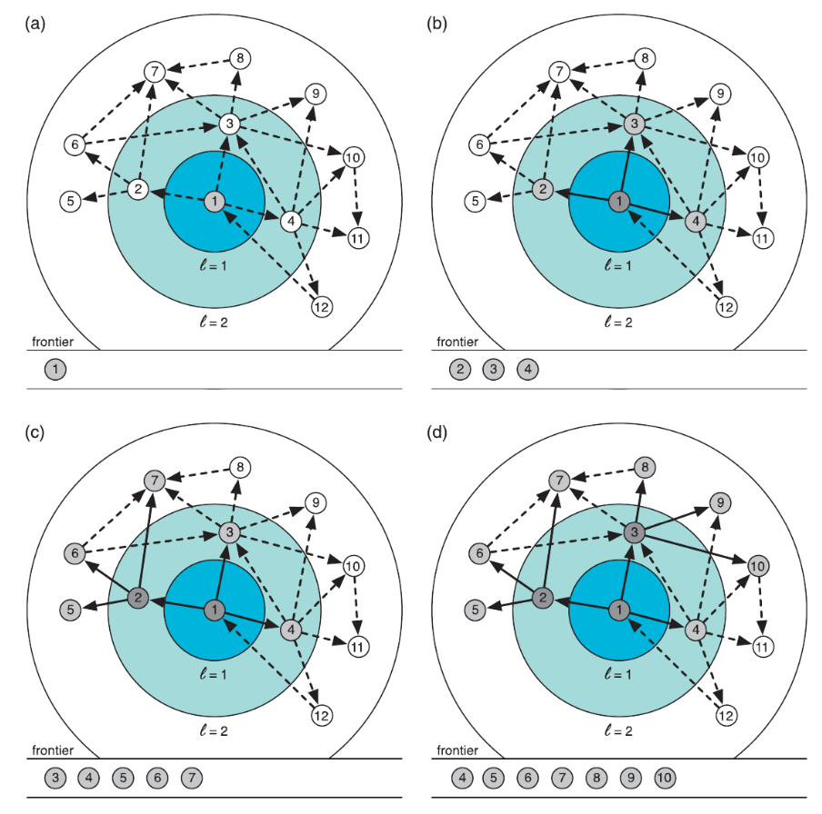
Example: Directed case
- The procedure is analogous for directed networks, except that we only reach nodes through directed paths from the source.1
Depth-First Search (DFS)
What is DFS?
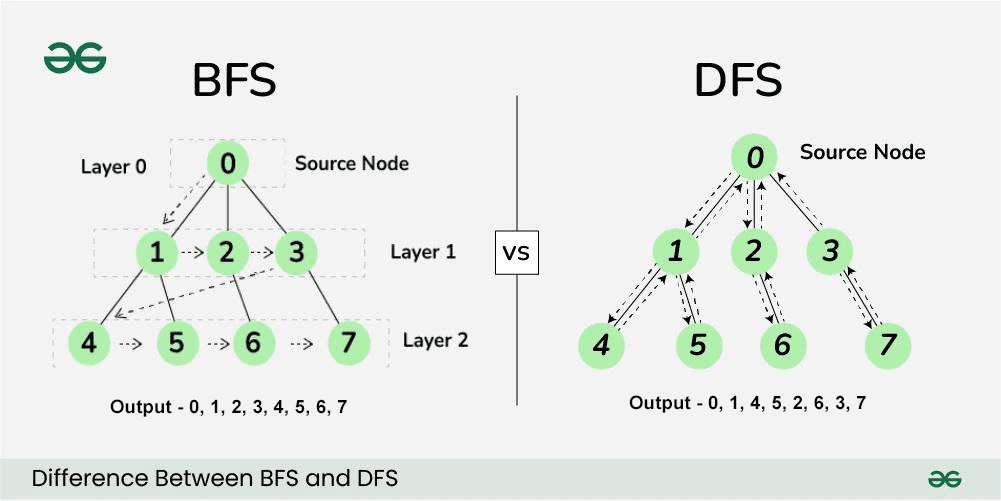
Unlike Breadth-First Search (BFS), which explores all neighbors at the current depth before moving to the next layer, Depth-First Search (DFS) explores as far as possible along each branch before backtracking.
- Depth-First Search (DFS) is a graph traversal algorithm that:
- Explores as far as possible along each branch before backtracking
- Mimics navigating a maze: pick a path, continue until a dead end, then backtrack to the last junction and try another route
Core Idea
Given a graph \(G = (V, E)\) and a starting node \(s\), DFS systematically visits every reachable node by always advancing to an unvisited neighbor before retreating.
The key data structure is a stack (either explicit, or implicitly via recursion).
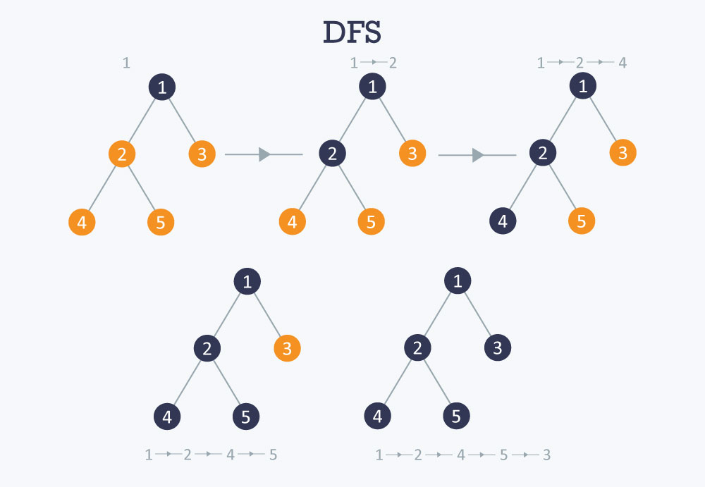
Pseduo code for DFS
A stack is a list where you can only add and remove from the top, the last item you put in is the first one you take out (LIFO). In DFS, this means you always explore the most recently discovered neighbor next, which is what drives the algorithm deep before it goes wide.
pop removes and returns the top item from the stack, so after a pop, that item is gone from the stack and you’re “holding it” to work with.
DFS(graph, start):
    stack ← [start]
    visited ← {}

    while stack is not empty:
        node ← pop(stack)

        if node not in visited:
            visited.add(node)
            process(node)

            for each neighbor of node:
                if neighbor not in visited:
                    push(stack, neighbor)
The one thing that makes it DFS specifically is the stack (last-in, first-out), swapping it for a queue turns this into BFS.
Example
Consider this undirected graph:
    A
   / \
  B   C
 / \   \
D   E   F
Represented as an adjacency list:
graph = {
    'A': ['B', 'C'],
    'B': ['A', 'D', 'E'],
    'C': ['A', 'F'],
    'D': ['B'],
    'E': ['B'],
    'F': ['C']
}
Starting DFS at A, one possible traversal order is:
| Step | Node Visited | Stack (after step) |
|---|---|---|
| 1 | A | [B, C] |
| 2 | B | [D, E, C] |
| 3 | D | [E, C] |
| 4 | E | [C] |
| 5 | C | [F] |
| 6 | F | [] |
Visit order: A → B → D → E → C → F
DFS Tree and Edge Types
When DFS runs on a graph, it naturally produces a DFS tree. Edges in the original graph fall into one of four categories:
| Edge Type | Description |
|---|---|
| Tree edge | Edge used to discover a new node |
| Back edge | Edge to an ancestor in the DFS tree (indicates a cycle) |
| Forward edge | Edge to a descendant (directed graphs only) |
| Cross edge | Edge between nodes in different DFS subtrees (directed graphs only) |
Complexity
| Complexity | |
|---|---|
| Time | \(O(V + E)\), every node and edge is visited once |
| Space | \(O(V)\), for the visited set and recursion stack |
For dense graphs where \(E \approx V^2\), this simplifies to \(O(V^2)\).
Key Applications
Cycle detection: a back edge in the DFS tree means the graph has a cycle.
Topological sort: for a directed acyclic graph (DAG), output nodes in reverse order of their finish times.
Connected components: run DFS from each unvisited node; each separate DFS call finds one component.
Strongly connected components (SCCs): Kosaraju’s and Tarjan’s algorithms both build on DFS.
Solving mazes and puzzles: DFS naturally models exhaustive search with backtracking.
DFS vs. BFS
| DFS | BFS | |
|---|---|---|
| Data structure | Stack | Queue |
| Explores | Deep first | Wide first |
| Shortest path? | No (unweighted) | Yes (unweighted) |
| Memory usage | \(O(depth)\) | \(O(width)\) |
| Good for | Cycle detection, topological sort, SCCs | Shortest paths, level-order traversal |