The Learning-on-Graphs Problem
Why standard MLPs & CNNs fail on graphs: and the symmetry that fixes it
Big picture: learning on graphs
Source: Unless otherwise stated, the information and images in this section come from “Sanchez-Lengeling, et al., A Gentle Introduction to Graph Neural Networks, Distill, 2021.” https://distill.pub/2021/gnn-intro/ and Machine Learning with PyTorch and Scikit-Learn, Sebastian Raschka, Yuxi Liu, Vahid Mirjalili, Dmytro Dzhulgakov, February-2022, Packt Publishing
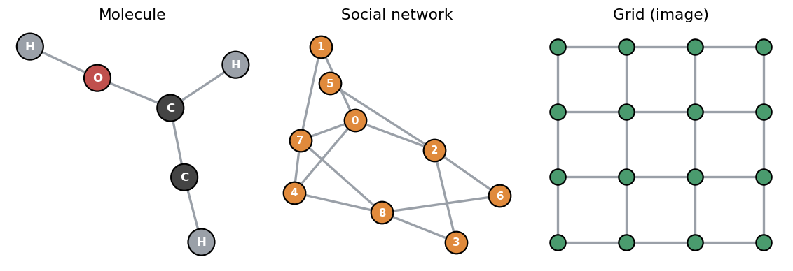
As we know: Graphs are everywhere
- Molecules: atoms are nodes, bonds are edges
- Social networks: people are nodes, friendships are edges
- Also: citation networks, road maps, recommender systems, knowledge graphs, the web
- Common thread → the relationships matter as much as the entities
Graph data
- A graph carries two things at once:
- Structure: who is connected to whom
- Features: what each node is
- The trouble: our usual tools (MLPs, CNNs) assume things a graph never gives us
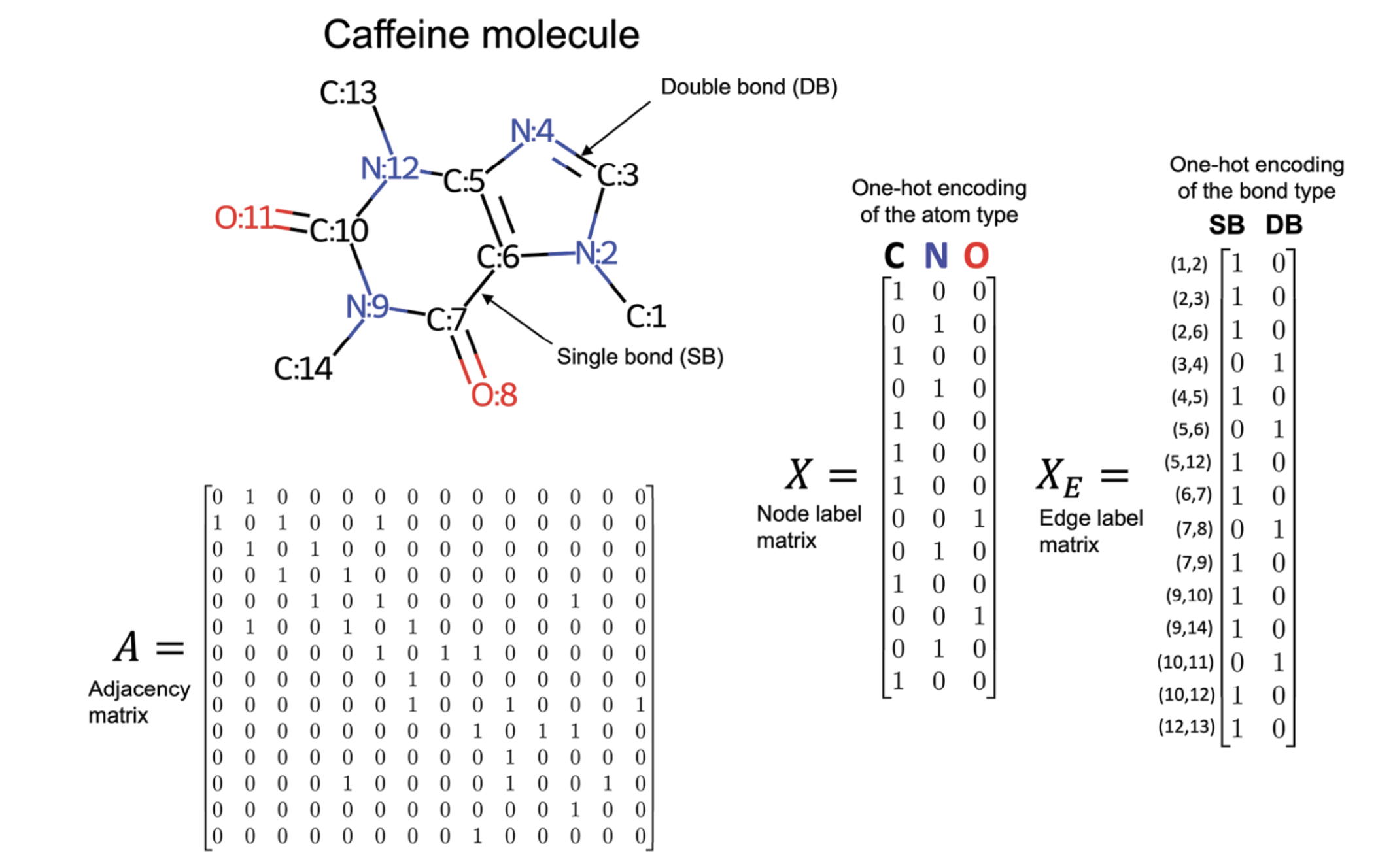
Another example: Molecules
Molecules can be represented as undirected graphs. - Node label matrix: each row is a one-hot encoding of the atom type. - Edge label matrix: each row is a one-hot encoding of the bond type.
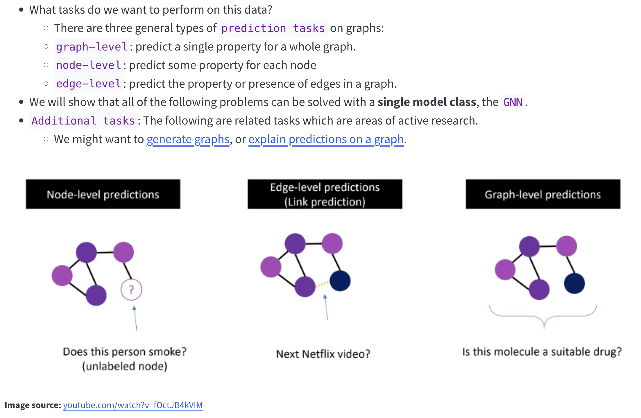
Graph Learning tasks
- Goal: learn a function whose input is an entire graph
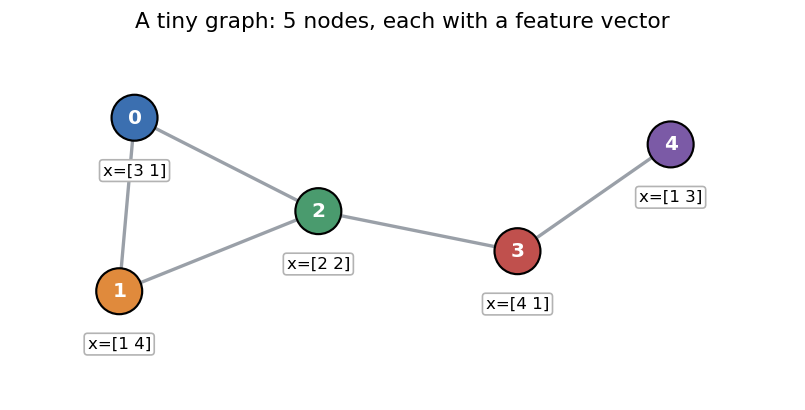
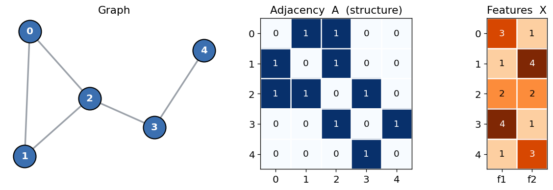
Simple example of a graph
- Nodes \(V\), edges \(E\), with \(n = |V|\) nodes
- Adjacency matrix \(A \in \{0,1\}^{n \times n}\) → \(A_{ij}=1\) when \(i\) links to \(j\)
- Feature matrix \(X \in \mathbb{R}^{n \times d}\) → row \(i\) = features of node \(i\)
- A model must consume both \(A\) and \(X\): together
Motivations: Why MLPs fail
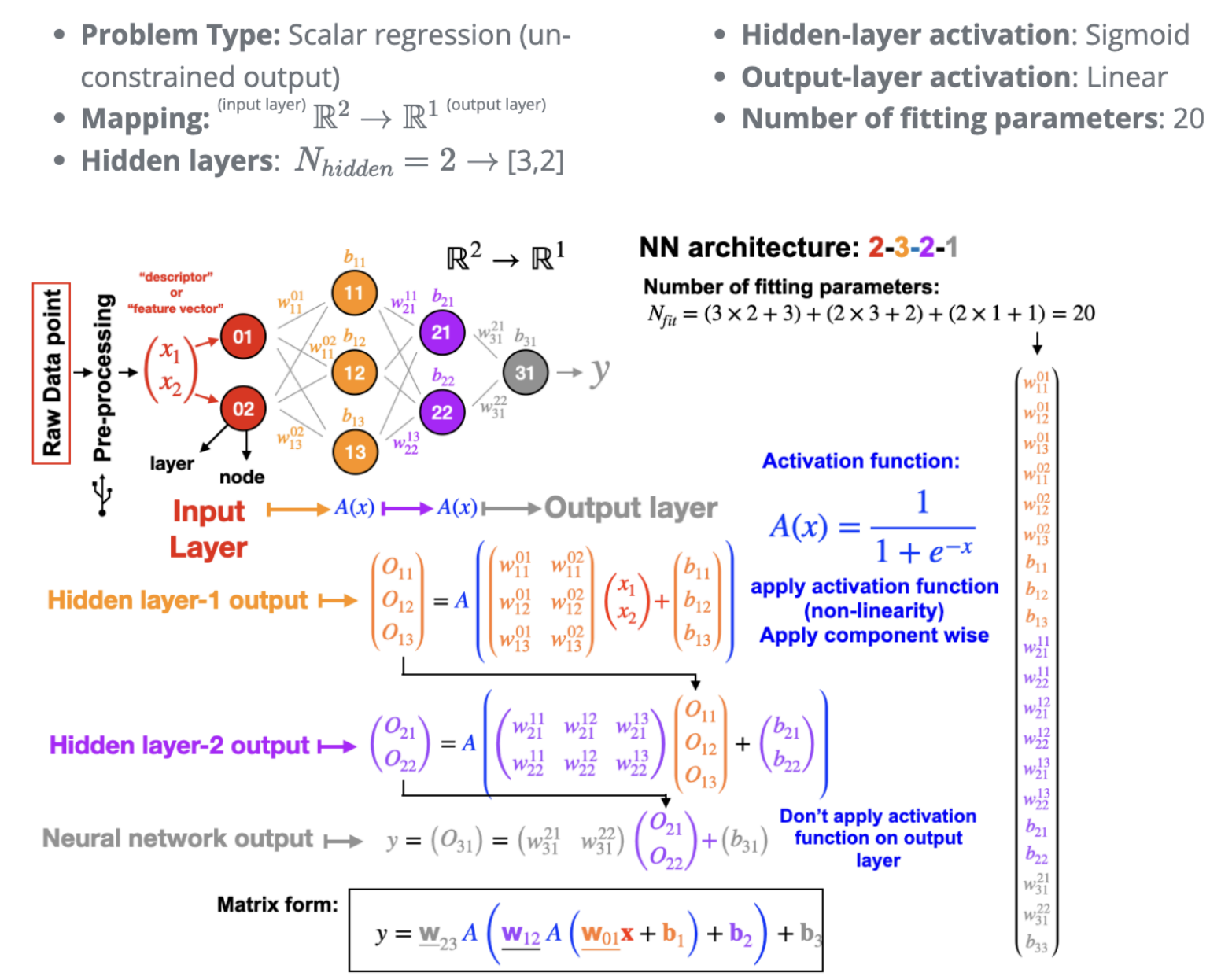
Recall the standard MLP
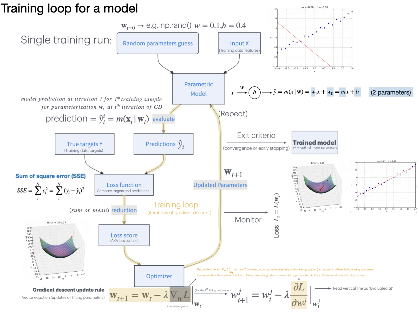
Recall how we train them
An MLP wants a fixed, ordered vector
- An MLP maps a fixed-length vector → output
- To feed a graph we would have to flatten it into one long row
- e.g. stack the adjacency matrix + features into a vector
- Sounds fine… until two problems appear immediately
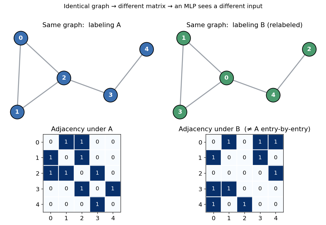
Problem 1: node ordering is arbitrary
- Node labels \(0,1,2,\dots\) are just names we picked: no natural meaningful order exists
- Node naming is a human convention, not a property of the graph
- human conventions have no place in a well constructed model, models should be arbitrary
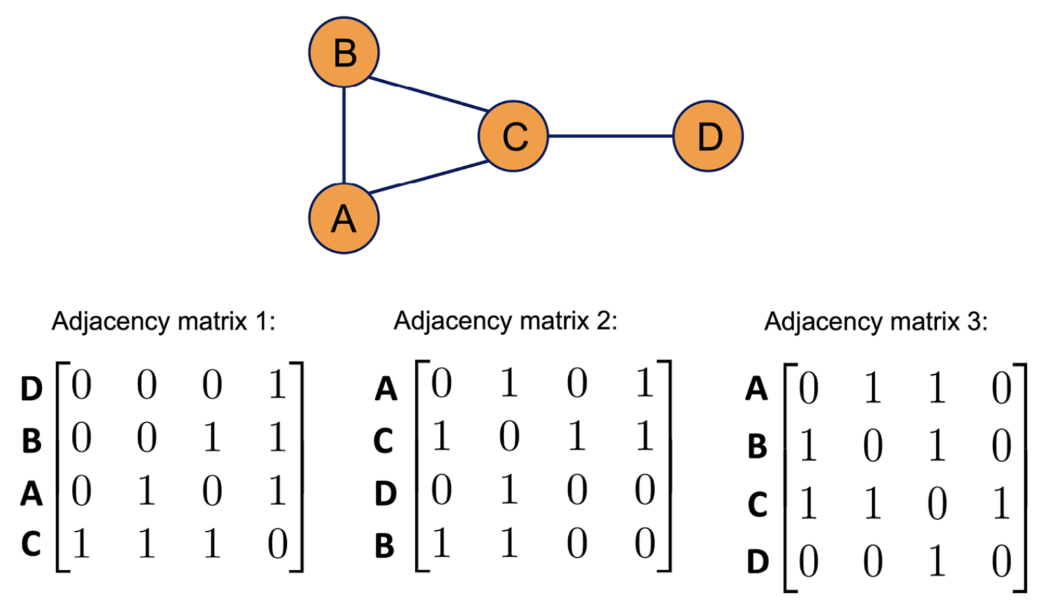
- Reorder the nodes → rows & columns of \(A\) shuffle
- Same graph, different matrix → the MLP sees a different input
- So an MLP could give two different answers to the identical graph
Problem 2: graphs come in different sizes
- An MLP’s input dimension is fixed at training time
- Real datasets mix sizes: a molecule with 5 atoms and one with 50, same dataset
- A flattened adjacency has size \(n^2\): it changes with every graph
- No single input layer can fit them all
- Also computational complexity is \(O(n^2)\) which is problematic for large graphs
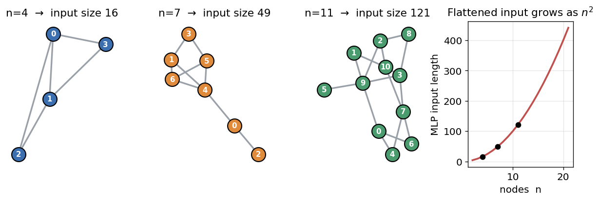
The deeper issue
- Flattening destroys structure and invents an order that isn’t real
- What we actually want:
- an answer that does not depend on the labeling
- An MLP has no way to know two labelings methods are the same graph
Why CNNs fail
Although they almost work
Jargon alert: Inductive Bias
Inductive bias is the set of assumptions built into a model that make it prefer some generalizations over others, letting it extend from the finite data it has seen to inputs it hasn’t.
- Any finite dataset can be fit by infinitely many functions: inductive bias is what makes a model prefer some over others.
- It’s baked into the architecture before training: a prior belief about how the world is structured, not something learned from data.
- Without it, generalization is impossible: nothing to favor one explanation over another
Examples of inductive bias:
- CNN: “nearby pixels matter, and a pattern means the same thing anywhere” → locality + translation equivariance
- GCN: “connected nodes tend to be similar” → relational / graph structure
- MLP: “assume almost nothing” → maximally flexible, needs the most data
The core trade-off:
- Strong bias → learns from less data, but assumes more (fails if the assumption is wrong)
- Weak bias → very flexible, but data-hungry
- The right inductive bias is a head start: match it to your data → fewer examples, better generalization; mismatch it → the model fights the data.
CNNs are made for grids
- A CNN leans on two facts about images:
- Fixed neighborhoods: every pixel has the same \(3\times3\) neighborhood shape
- Translation: one filter slides everywhere (weight sharing)
- That is a powerful, correct inductive bias: for grid data (essentially spatial correlation)
An image is a graph
- Pixels are nodes; each pixel connects to its neighbors
- It is just a very regular graph: a grid
- Every interior pixel has exactly 4 neighbors, always in the same positions
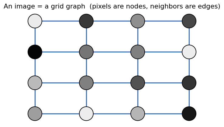
Example: Images as graphs
This may seem trivial, but there’s a strong connection between convolutional neural networks and graph neural networks.
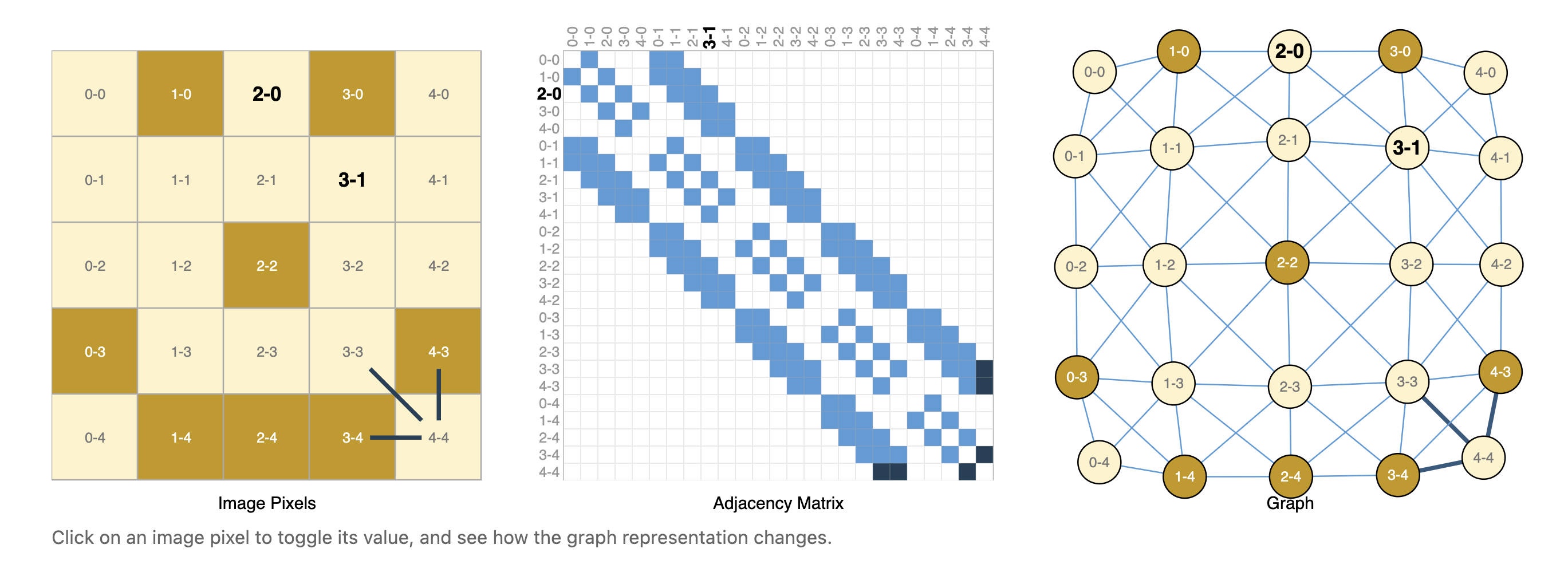
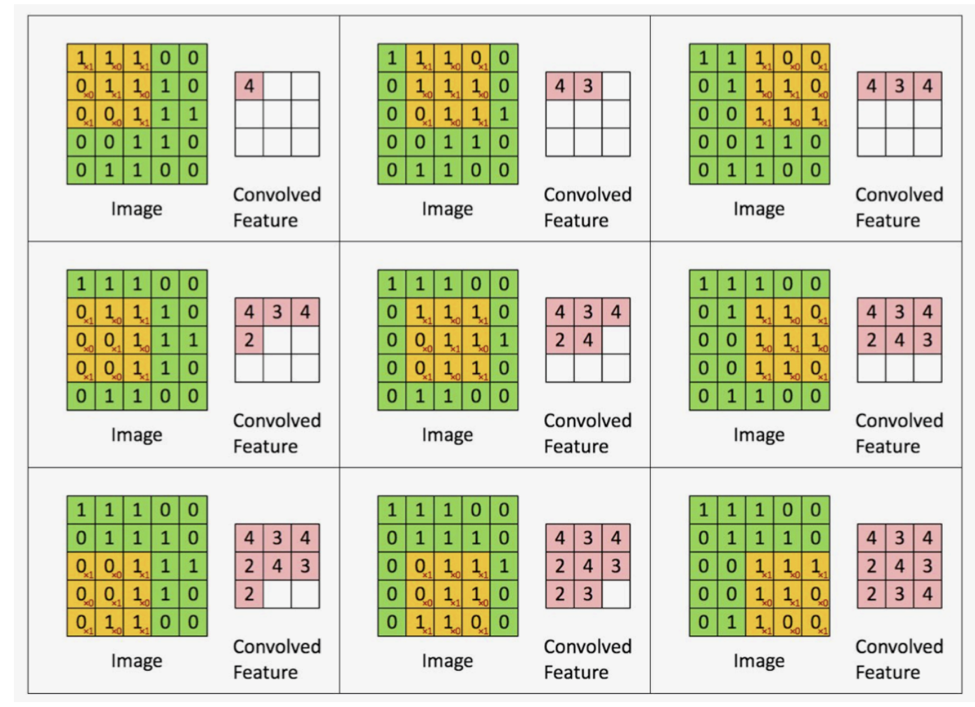
Operation-1: Convoluition operation
Note that the convolution operation extracts local information, where local in this context means around a central pixel.
Operation-2: Pooling
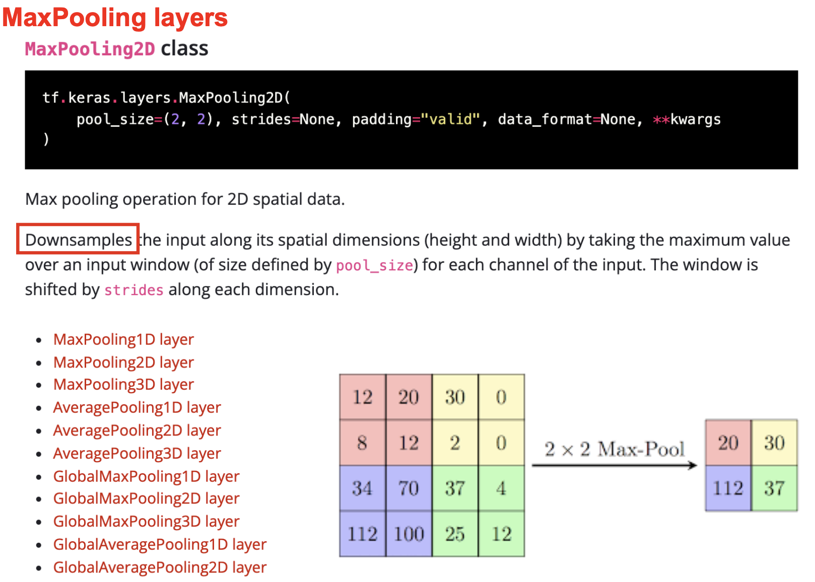
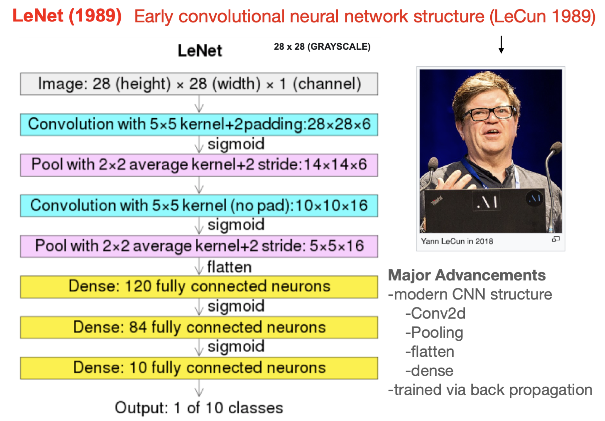
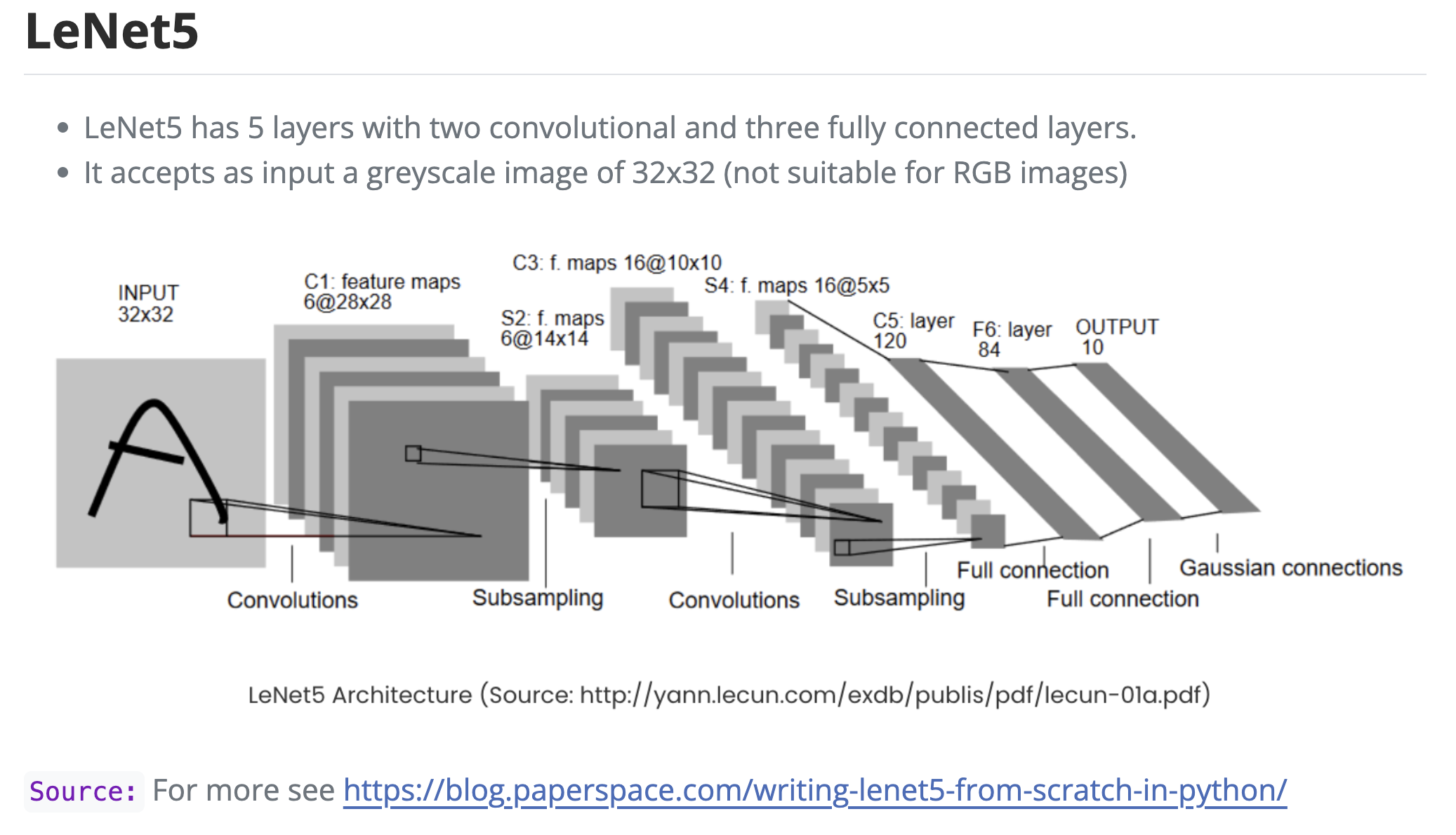
Recall the CNN Model
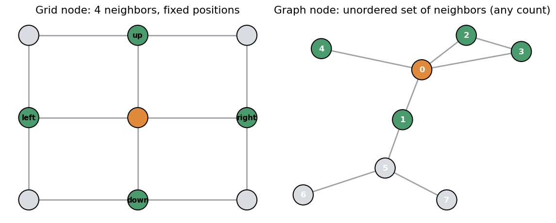
General graphs break the grid assumptions
- Neighborhood size varies: one node has 2 neighbors, another has 17
- No canonical neighbor order: which neighbor is “up”? “left”? undefined
- A \(3\times3\) filter has labeled slots (top-left, top, …); a graph node has an unordered set
- “One weight per position” doesn’t even make sense on a graph
We need a new inductive bias for graphs
- Not “slide a fixed filter across a grid”
- Instead: combine each node with its neighbors in a way that ignores order and count
- That requirement has a precise name → permutation symmetry
- Permutation symmetry is the property that an object stays fundamentally unchanged when its elements are relabeled or reordered:
- for a graph, permuting the node labels via A ↦ PAP⊤ yields the same graph,
- so any function of it should give the same answer (invariance)
- OR a correspondingly systematicallyrelabeled one (equivariance).
- for a graph, permuting the node labels via A ↦ PAP⊤ yields the same graph,
- Permutation symmetry is the property that an object stays fundamentally unchanged when its elements are relabeled or reordered:
Equivariance or invariance
Jargon alert: Equivariance vs. Invariance
- Common transformations to data:
- Translation: shift the input
- Rotation: rotate the input
- Scale: zoom in or out
- Shear: distort the input
- Permutation: shuffle the order of the input
Equivariant: transform the input → the output transforms the same way.
Invariant: transform the input → the output doesn’t change at all.
- Formally, for a transformation
T(e.g. a spatial shift):- Equivariance:
f(T(x)) = T(f(x)): “move the input, the answer moves with it” - Invariance:
f(T(x)) = f(x): “move the input, the answer stays put”
- Equivariance:
Either of these is an acceptable condition: in one case, the transformation has no effect on the output and is therefore irrelevant; in the other, the transformation systematically alters the output, which is also reasonable, because it remains a useful output.
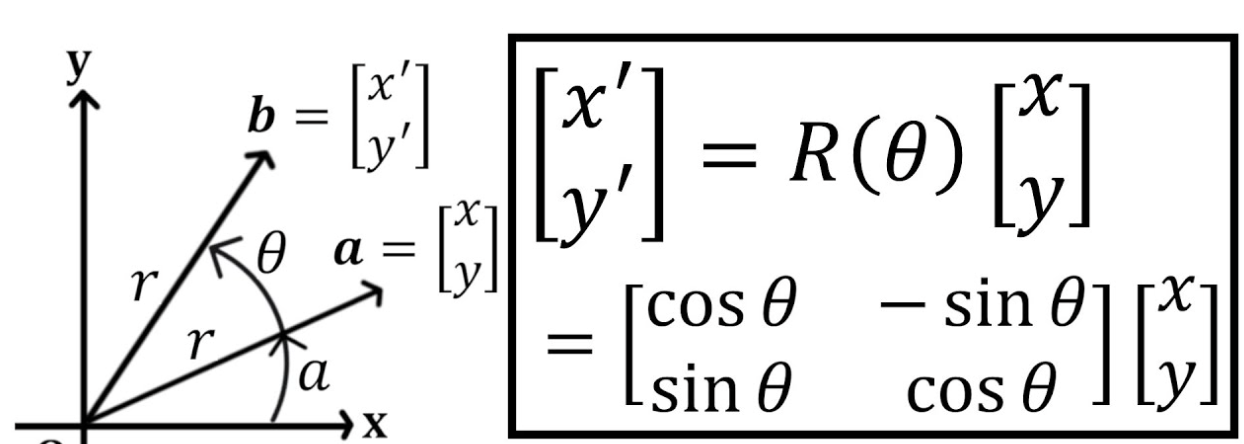
Example transformation:The Rotation Matrix
A rotation matrix
R(θ)turns a vector by angleθabout the origin: it changes direction while preserving length.
- Think of it as spinning the coordinate axes by
θ; every vector rotates rigidly with them. - It preserves lengths and angles: a rotation never stretches, shrinks, or reflects.
- Columns of
Rare just where the unit axes land after the turn.
2-D rotation, then a simple 90° example:
\[ R(\theta)=\begin{bmatrix}\cos\theta & -\sin\theta\\[2pt] \sin\theta & \cos\theta\end{bmatrix}, \qquad R(90^\circ)=\begin{bmatrix}0 & -1\\ 1 & 0\end{bmatrix} \]
\[ R(90^\circ)\begin{bmatrix}1\\0\end{bmatrix}=\begin{bmatrix}0\\1\end{bmatrix} \qquad\text{— the } x\text{-axis rotates onto the } y\text{-axis.} \]
Important properties:
- Orthogonal: \(R^{\top}R = I\), so the inverse is the transpose, \(R^{-1}=R^{\top}=R(-\theta)\).
- \(\det(R)=+1\): a proper rotation (orientation preserved); \(\det=-1\) would be a reflection.
- Rotations compose by adding angles: \(R(\alpha)\,R(\beta)=R(\alpha+\beta)\).
Example transformation: The Permutation Matrix
A permutation matrix
Pis a square matrix of 0s and 1s with exactly one 1 in each row and each column: it reorders the entries of whatever it multiplies.
- Think of it as the identity matrix
Iwith its rows shuffled. - Left-multiply
Px→ reorders the rows (entries) of a vector; right-multiply reorders columns. - It only rearranges: never scales, mixes, or destroys information.
Simple example: cyclically shift a 3-vector:
\[ P=\begin{bmatrix}0&1&0\\0&0&1\\1&0&0\end{bmatrix}, \qquad P\begin{bmatrix}a\\b\\c\end{bmatrix}=\begin{bmatrix}b\\c\\a\end{bmatrix} \]
- Row 1 =
[0 1 0]picks the 2nd entry, row 2 picks the 3rd, row 3 picks the 1st.
Important properties:
- Orthogonal: \(P^{\top}P = I\), so the inverse is just the transpose, \(P^{-1}=P^{\top}\).
- \(\det(P)=\pm 1\); a product of permutation matrices is again a permutation matrix.
Why we care (graphs): relabeling a graph’s nodes is exactly \(A \mapsto P A P^{\top}\): the tool we need to state permutation equivariance for GNNs.
Permutating a matrix
- Vector (one axis):
Pxreorders the entries. - Matrix (two axes):
PAreorders the rows,AP^⊤reorders the columns →PAP^⊤does both.
Why both sides?
- In an adjacency matrix,
A[i,j]= “edge from nodeito nodej”: both axes are indexed by nodes. - Renaming rows only would leave the columns inconsistent;
P … P^⊤renumbers both axes the same way, keeping every edge intact.
Nice fact:
Pis orthogonal, so \(P^{\top}=P^{-1}\) → \(PAP^{\top}=PAP^{-1}\), a change of basis where the “coordinates” are just node labels.
One-liner: one P reorders a list; P … P^⊤ reorders a table indexed by the same objects on both sides.
The general pattern \(M \mapsto S M S^{-1}\) (matrix on one side, its inverse on the other) is a similarity transformation, and \(M\) and \(S M S^{-1}\) are similar matrices. This is the change-of-basis operation: M and \(SMS^\{-1\}\) represent the same linear map in different bases. Similar matrices share eigenvalues, determinant, trace, and rank.
Is \(Px\) a Change of Coordinates?
Yes:
Pxis a change of basis, but the most rigid kind: it only reorders the axes (feature dimensions), never rotates, scales, or mixes them.
- A general basis change
x ↦ Sxcan blend axes: e.g. a new axis =0.3·x_1 + 0.7·x_5. - A permutation
x ↦ Pxis the special case where each new coordinate is exactly one old coordinate: pure relabeling, information-preserving.
One subtlety: active vs. passive:
- Passive: the point stays put; you just rename which feature is “first,” “second,” … (reorder the axes).
- Active: the entries physically move to new slots.
- Same numbers result: but relabeling axes by
P= moving the point by \(P^{-1}=P^{\top}\) (the two are inverses).
Why it matters for graphs:
- Relabeling nodes must only reorder: it can’t mix two nodes into a blend.
- That restriction is exactly what makes it a symmetry (object unchanged), not an arbitrary coordinate change: and why
Pxgeneralizes to \(PAP^{\top}\).
One-liner: Px reorders the axes; it’s a change of basis stripped down to pure relabeling: which is precisely what a symmetry needs.
Permuting nodes = relabeling
- A permutation just renames nodes: represented by a permutation matrix \(P\)
- \(P\) has exactly one \(1\) per row and per column
- Under a relabeling:
- Features: \(X \to PX\)
- Adjacency: \(A \to P A P^{\top}\)
- The graph itself is unchanged: only our bookkeeping moved
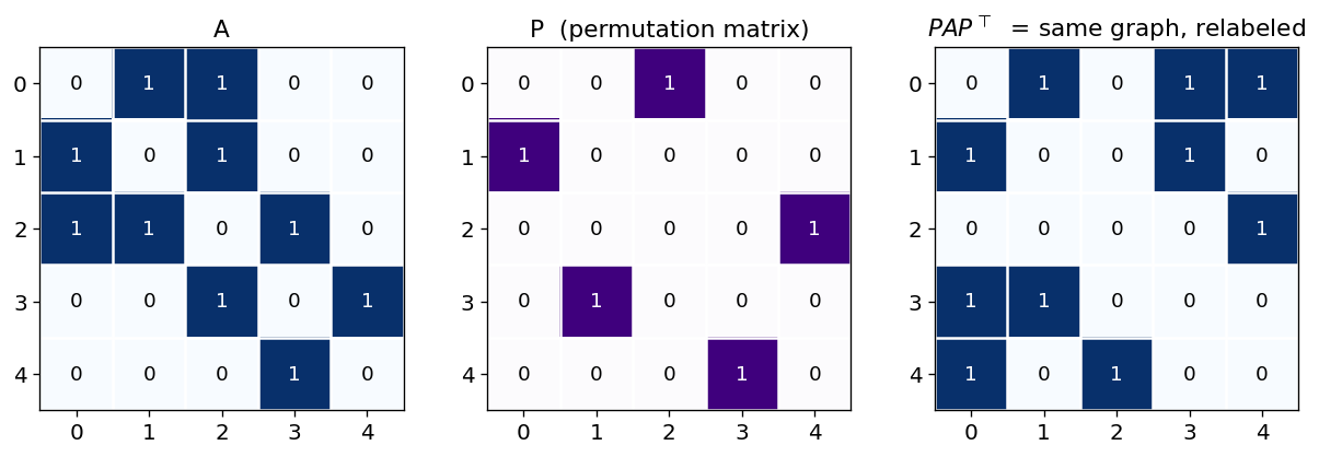
Adjacency matrix is not invariant to relabeling
- This means that the adjacency matrix will change if we relabel the nodes.
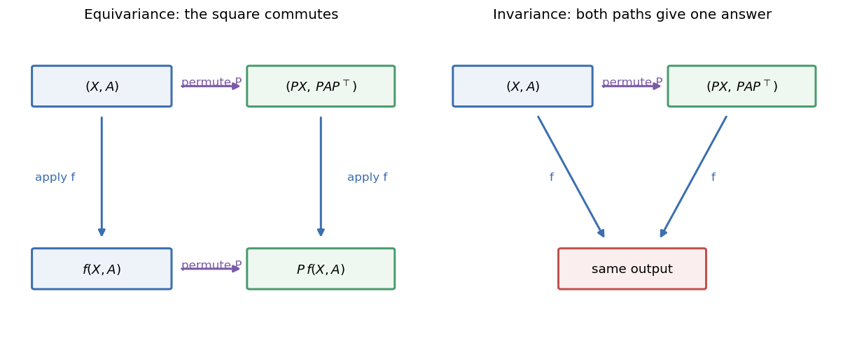
Two symmetries we actually want
- Permutation invariant: for graph-level outputs
- relabel the nodes → output is unchanged
- \(f(PX,\,PAP^{\top}) = f(X, A)\)
- “How many nodes there are in the graph?” can’t depend on labeling
- Permutation equivariant: for node-level outputs
- relabel the nodes → outputs relabel the same way
- \(f(PX,\,PAP^{\top}) = P\,f(X, A)\)
- each node’s prediction travels with its node
Injecting invariance
- To get a graph-level number → sum (or mean) over all nodes
- A sum ignores order → invariant
- This is exactly why GNNs use symmetric aggregation (sum / mean / max)
Example: Mean Aggregation
- Simplest possible graph operation → replace each node’s feature with the mean over its neighbors (plus itself)
Mean aggregation summarizes a node’s neighborhood by averaging the feature vectors of its neighbors: one representative “average neighbor” vector, regardless of how many neighbors there are.
- Permutation-invariant: the average doesn’t depend on the order neighbors are listed.
- Size-normalized: dividing by the neighbor count keeps the scale comparable across high- and low-degree nodes.
- Captures the neighborhood’s “typical” / central feature: but discards how many neighbors and any outliers.
Equation: aggregated message at node i:
\[ h_{\mathcal{N}(i)} \;=\; \frac{1}{|\mathcal{N}(i)|}\sum_{j \in \mathcal{N}(i)} h_j \]
- \(\mathcal{N}(i)\) = the set of neighbors of node
i - \(|\mathcal{N}(i)|\) = number of neighbors (the degree)
- \(h_j\) = feature vector of neighbor
j
Example: Mean Aggregation
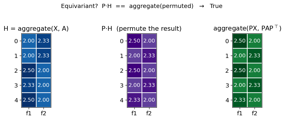
- Invariant to reordering a node’s neighbors: the average forgets order, so a neighborhood’s aggregated vector is the same regardless of how its neighbors are listed (invariance forgets where).
- Equivariant to relabeling the whole graph’s nodes: renumber all nodes and the per-node outputs just get reindexed the same way:
AGG(PAP⊤, PX) = P·AGG(A, X)(equivariance preserves where).
Equivariance vs. Invariance: Which & When
We actually need respect permutation symmetry: the difference is whether node identity still matters at the output.
- Equivariant: the reordering is tracked and carried through; outputs get relabeled to match. Nothing lost.
- Invariant: the reordering is irrelevant; the output is unchanged because labels no longer carry meaning.
The output’s structure dictates which you need:
| Output type | Required property | Why |
|---|---|---|
| Per-node (node labels, embeddings) | Equivariance | identity must travel with the permutation |
| Whole-graph (one prediction) | Invariance | no node to label → relabeling can’t matter |
Realized in a standard modern GCN:
- GCN layers \(\rightarrow\) equivariant. Each layer computes \(\sigma(\hat{A}XW)\) per node and carries identity through: \(f(PAP^{\top},\, PX) = P \cdot f(A, X)\). Stacking keeps the whole trunk equivariant.
- Readout \(\rightarrow\) invariant (only if graph-level). A final pool (mean/sum/max over all nodes) collapses identity \(\rightarrow\) one order-independent graph vector.
The design rule:
- Equivariant middle, invariant cap: preserve “where” as long as the task needs it, discard it exactly when it stops mattering.
- Invariant too early \(\rightarrow\) throws away node info you still need.
- Equivariant at a graph-level output \(\rightarrow\) leaks the arbitrary node ordering into the prediction.
One-liner: stack equivariant layers; add an invariant readout only when the task is about the whole graph.
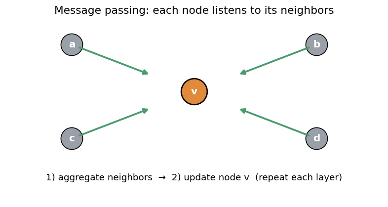
Looking ahead: The GNN recipe
- Repeat, layer by layer:
- each node aggregates its neighbors’ features: symmetric, so permutation-safe
- each node updates itself with a small learnable function: shared across all nodes
- Stack layers → information flows farther across the graph
- Weight sharing across nodes ↔︎ the same idea as translation weight-sharing in CNNs
Why this is the right bias
- It encodes a true fact about the world → node names are meaningless
- A model with this bias cannot be fooled by reordering
- Operations act per-node / per-neighbor \(\rightarrow\) one model handles any size graph
Summary of key points
- Graphs have no fixed ordering and variable neighborhoods → MLPs & CNNs don’t fit
- The right inductive bias is permutation symmetry:
- invariance for graph-level tasks · \(f(PX, PAP^\top)=f(X,A)\)
- equivariance for node-level tasks · \(f(PX, PAP^\top)=P f(X,A)\)
- Get it for free with symmetric neighbor aggregation (sum / mean / max)
- Always use features and structure together
- This is the foundation of Graph Neural Networks: up next