What changes when edges carry intensity AND/OR point one way.
“The simple graph is where we learn the concepts; the weighted directed network is where we meet reality.”
Topics topics
Source: Unless otherwise stated, content comes primarily from chapter-4 in the textbook1
Chapter-4: Directions and Weights from the textbook1
Directed Networks
The Web
Review: Eigen-values
Eigen-centrality
PageRank
Weighted Networks
Information and Misinformation
Co-occurrence Networks
Weight Heterogeneity.
Utility plotting function
# === Lecture setup: run this cell first ======================================# Import necessary librariesimport networkx as nx # For building and manipulating networksimport numpy as np # For numerical operations (not always needed, but handy)import matplotlib.pyplot as plt # For plotting graphs# Enable inline plotting in notebooks%matplotlib inline# Print out the NetworkX version for reproducibility/debuggingprint("NetworkX", nx.__version__)# Update matplotlib parameters for consistent, clean visuals throughout the deckplt.rcParams.update({"figure.figsize": (6.4, 4.1), # Set a convenient figure size"figure.dpi": 115, # Reasonable DPI for screenshots or projection"font.size": 11, # Base font size for plot text"axes.titlesize": 12.5, # Larger title font"savefig.bbox": "tight", # Tighter bounding box when saving figures})# Define a color palette for consistency and accessible contrast throughout the slidesBLUE ="#4C72B0"ORANGE ="#DD8452"RED ="#C44E52"GREEN ="#55A868"GREY ="#8C8C8C"def draw_graph( G, pos=None, node_color=BLUE, title=None, ax=None, show_weights=False, node_size=950, font_color="white", arrowsize=20, edge_color="#4d4d4d", width=1.8, edge_labels=None, highlight_edges=None, curved=False, label_pos=0.5, font_size=11,):""" Draw a tidy, publication-ready visualization of a NetworkX graph. Parameters: ----------- G : networkx.Graph or networkx.DiGraph The graph to plot. pos : dict (optional) Node positions, as a dict: {node: [x, y]}. If None, spring layout is used. node_color : str or list Color of nodes (all or per-node). title : str (optional) Title for the plot. ax : matplotlib.axes.Axes (optional) The axes to plot on. If None, a new figure and axes will be created. show_weights : bool Whether to show edge weights (if present). node_size : int Size of nodes. font_color : str Node label font color. arrowsize : int Size of arrow heads. edge_color : str or list Color for the edges. width : float Width of edges. edge_labels : dict (optional) Custom labels for edges. highlight_edges : list (optional) List of edges to highlight in red (e.g., for emphasis). curved : bool Whether to draw curved edges. label_pos : float Position of edge labels. font_size : int Node label font size. """ created =False# Track if we need to plt.show() at end# Create axes if not providedif ax isNone: fig, ax = plt.subplots() created =True# Use spring layout if not providedif pos isNone: pos = nx.spring_layout(G, seed=7)# Determine if directed for correct arrow style/behavior directed = G.is_directed()# Connection style for drawing arrows/curves (visually clearer for directed/curved) conn ="arc3,rad=0.12"if (curved or directed) else"arc3,rad=0.0"# Draw nodes nx.draw_networkx_nodes( G, pos, node_color=node_color, node_size=node_size, edgecolors="white", # white border for visibility linewidths=1.5, ax=ax )# Draw edges (arrows for directed) nx.draw_networkx_edges( G, pos, edge_color=edge_color, width=width, arrows=True, arrowsize=arrowsize, connectionstyle=conn, node_size=node_size, ax=ax )# Optionally, highlight specific edges if requested (e.g., to show a path)if highlight_edges: nx.draw_networkx_edges( G, pos, edgelist=highlight_edges, edge_color=RED, width=3.4, arrows=True, arrowsize=arrowsize +2, # make the highlight more visible connectionstyle=conn, node_size=node_size, ax=ax )# Draw node labels nx.draw_networkx_labels( G, pos, font_color=font_color, font_weight="bold", font_size=font_size, ax=ax )# Prepare edge labels (default to 'weight' attr if asked)if show_weights and edge_labels isNone: edge_labels = { (u, v): d.get("weight", "") for u, v, d in G.edges(data=True) }# Draw edge labels (if present)if edge_labels: nx.draw_networkx_edge_labels( G, pos, edge_labels=edge_labels, font_size=10, label_pos=label_pos, bbox=dict(boxstyle="round,pad=0.15", fc="white", ec="none", alpha=0.85), ax=ax )# Add a title (if provided)if title: ax.set_title(title)# Clean up axes for that "slidedeck look" ax.axis("off")# Show plot if we created the figureif created: plt.tight_layout() plt.show()# Return the position (so we can reuse layout on later plots)return pos
NetworkX 3.6.1
Where we have been: Simple graphs
The simple graph is a beautiful idealization
The usual starting point of a network analysis class is the simple graph: edges are
binary, present or absent, and
symmetric, if \(a \rightarrow b\) exists, so does \(b \rightarrow a\).
An enormous amount of structural insight, degree distributions, clustering, components, small-world geometry, lives here. But for most real systems it is a drastic idealization:
Examples:
Importance of weights: A graph that records only whether two countries trade erases that the US–China flow is thousands of times larger than two smaller neighbours.
Importance of direction: A graph that records only whether neuron \(a\) connects to \(b\) erases that the signal flows \(a\to b\), not back.
Everything begins with the adjacency matrix
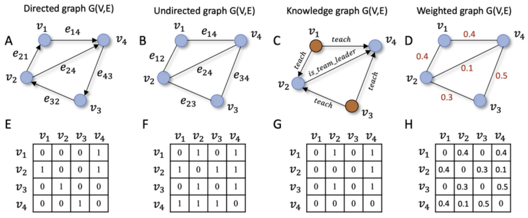
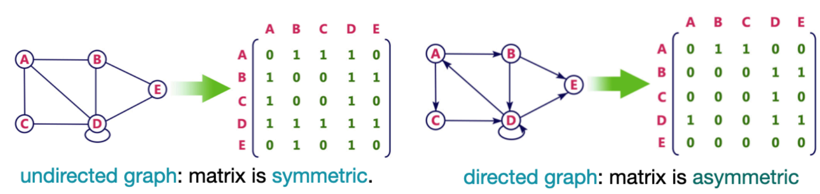
As we have seen, natural representation of any of these networks is the adjacency matrix\(\mathbf{A}\): a square array indexed by nodes whose entry \(A_{ij}\) records the edge from \(i\) to \(j\).
The two generalizations are exactly the relaxation of two matrix properties:
Weighting ⟶ \(\mathbf{A}\) is no longer binary; nonzero entries hold edge weights (flows, capacities, similarities, distances, …).
Directing ⟶ \(\mathbf{A}\) is no longer symmetric; \(A_{ij} \neq A_{ji}\) in general.
So much theory follows from linear algebra that it pays to see these as matrix properties.
Directed Networks
Un-directed case: In social networks, we often assume, even if it is not always true, that friendship is symmetric:
In many networks these symmetries do not hold;
i.e. a link has a particular direction, and may not be reciprocated.
You may follow Brad Pitt on twitter, but he probably doesn’t follow you.
Node degree is split into in and out degree and paths must respect link direction
In a directed network each node has an in-degree (number of incoming links) and an out-degree (number of outgoing links).
Weight and direction: Two independent “dimensions”
A network may have either, both, or neither property.
Weighted, edges carry a real-valued magnitude (a weight / strength) rather than mere presence.
Directed, edges are ordered pairs; \(a\to b\) is a different object from \(b\to a\), and either, both, or neither may exist.
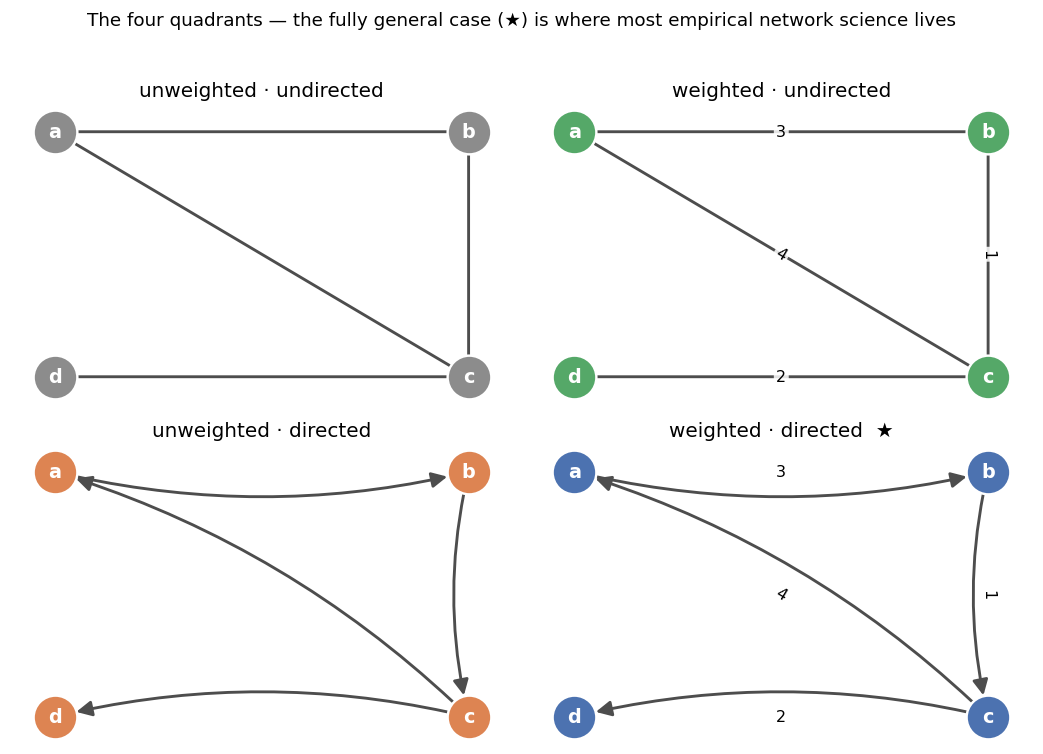
Knowing which quadrant your system occupies is the first analytical decision you make, and it should be deliberate, never a default. The cell below draws all four.
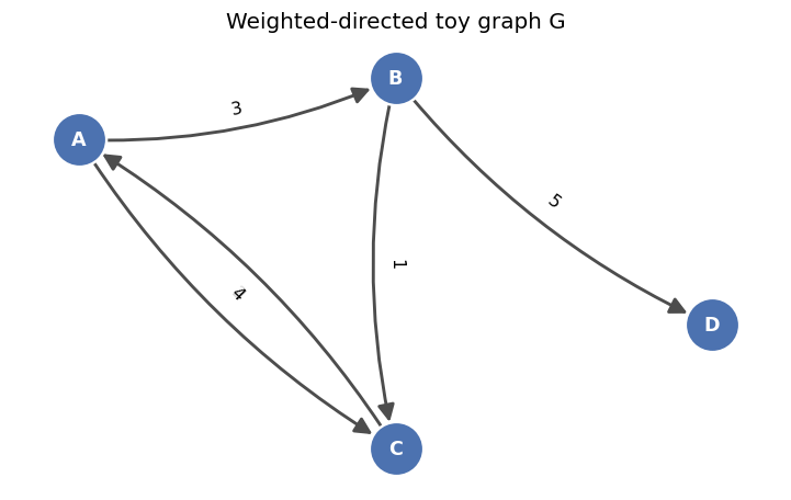
# The four quadrants of "richness", drawn on the same node layoutfig, axes = plt.subplots(2, 2, figsize=(9.2, 6.4))base = [("a","b"),("b","c"),("c","a"),("c","d")]layout = {"a":(0,1),"b":(1,1),"c":(1,0),"d":(0,0)}# (1) unweighted-undirectedG1 = nx.Graph(); G1.add_edges_from(base)draw_graph(G1, pos=layout, ax=axes[0,0], title="unweighted · undirected", node_color=GREY, node_size=750, font_size=12)# (2) weighted-undirectedG2 = nx.Graph()for (u,v),w inzip(base,[3,1,4,2]): G2.add_edge(u,v,weight=w)draw_graph(G2, pos=layout, ax=axes[0,1], title="weighted · undirected", node_color=GREEN, node_size=750, show_weights=True, font_size=12)# (3) unweighted-directedG3 = nx.DiGraph(); G3.add_edges_from(base)draw_graph(G3, pos=layout, ax=axes[1,0], title="unweighted · directed", node_color=ORANGE, node_size=750, font_size=12)# (4) weighted-directed (where most empirical work lives)G4 = nx.DiGraph()for (u,v),w inzip(base,[3,1,4,2]): G4.add_edge(u,v,weight=w)draw_graph(G4, pos=layout, ax=axes[1,1], title="weighted · directed ★", node_color=BLUE, node_size=750, show_weights=True, font_size=12)plt.suptitle("The four quadrants, the fully general case (★) is where most empirical network science lives", fontsize=11.5, y=1.02)plt.tight_layout(); plt.show()
Weight introduces intensity, direction introduces asymmetry
Weight = the magnitude of a tie. Direction = the asymmetry of a tie.
Together, weight and direction restore key information lost from
binarization (edge exists in adjacency matrix)
symmetrization (undirected edges)
The full description of a network is fundamentally more complex and nuanced than the simple case.
Key point: Weighted and directed networks require rethinking/defining even basic concepts and metrics
Simple notion
What it becomes
degree
in/out-degree and in/out-strength
connectivity
strong vs weak
one tidy centrality
a contested family (Katz, PageRank, HITS, …)
one clustering coefficient
a small family of definitions
density-based community
density vs flow
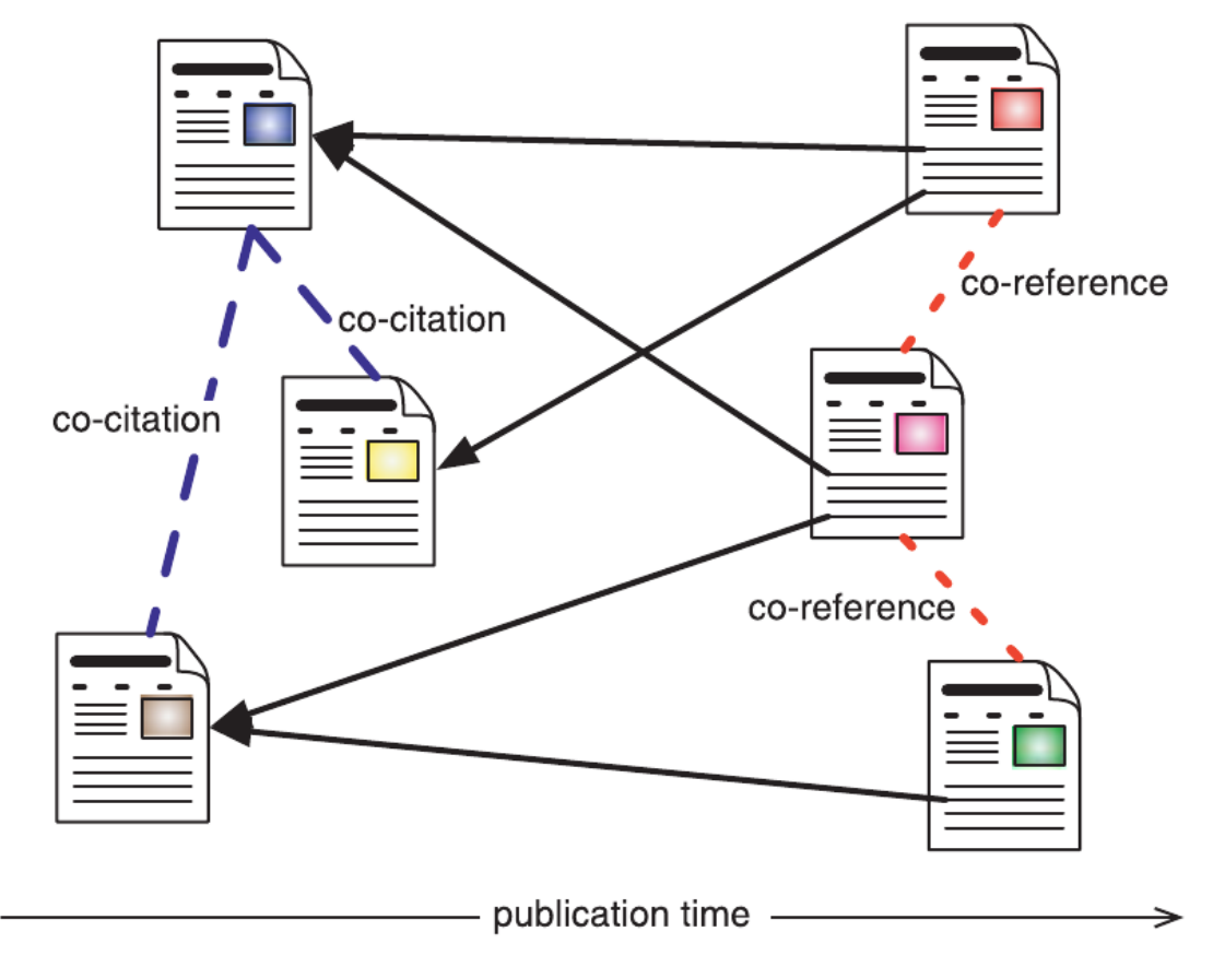
Example: Citation network
Node = A publication
Directed link = a given citation (black)
A citation indicates some kind of relationship between the content of the papers:
Key Point:
The meaning of an edge weight in a network is not inherent in the data, you, the modeler, must decide and clearly state it.
> A weight is not given by the data; its interpretation is chosen by the modeler.
Two common interpretations of edge weights:
Interpretation
What does a large weight mean?
Typical analysis goal
Affinity
Strong, similar, closely linked nodes
Seek paths with the largest total weight (e.g., maximize flow/similarity)
Cost
Far apart, expensive, or hard to traverse
Seek paths with the smallest total weight (e.g., minimize distance/time)
Affinity (strength, similarity, flow, capacity):
- Large weight ⇒ nodes are closer, more connected, more similar
- Example: Friendship strength, bandwidth, traffic volume
- Path/cluster selection: Prefer higher total weight
Cost (distance, expense, travel time):
- Large weight ⇒ nodes are further apart or harder to reach
- Example: Travel time, monetary cost, resistance
- Path/cluster selection: Prefer lower total weight
Whether you minimize or maximize when using algorithms (e.g., shortest path, community detection) depends on this choice.
Important metrics in directed and weighted networks
In directed and weighted network analysis, moving beyond simple unweighted or undirected metrics requires quantities that account for flow, asymmetry, and connection strength.
Node Degree and Strength Metrics
These quantities measure basic node activity and connectivity by adjusting for directionality and weights.
Definition: The sum of incoming edge weights (\(s_{in}\)) versus outgoing edge weights (\(s_{out}\)).
Significance: Crucial for identifying whether a node is a net consumer or net producer of flow within a network.
Centrality and Prestige Measures
These quantities determine the global importance or influence of a node within the network structure.
Katz Centrality:
Definition: Measures a node’s influence by counting all paths to it, penalizing longer paths via an attenuation factor \(\alpha\), and giving every node a baseline intrinsic bias \(\beta\).
Significance: The standard solution for ranking nodes in Directed Acyclic Graphs (DAGs) where standard eigencentrality collapses to zero.
PageRank Score (\(PR\)):
Definition: A variant of Hubbell/Katz centrality that scales a node’s transferred influence by its out-degree and introduces a random teleportation factor (\(1-d\)).
Significance: Evaluates the probability that a random walker will land on a node. Essential for directed web traffic, citation networks, and search engine indexing.
Weighted Betweenness Centrality (\(C_B^w\)):
Definition: The fraction of all weighted shortest paths between all pairs of nodes that pass through a specific node.
Significance: Identifies key “bottlenecks” or bridges controlling traffic flow. Because edge weights alter what is considered the “shortest path,” it often reveals entirely different bottlenecks than unweighted metrics.
Local Structure and Clustering
These quantities assess how tightly knit local neighborhoods are when accounting for direction and intensity.
Directed Clustering Coefficient (\(C^{dir}\)):
Definition: The ratio of directed triangles a node forms to the total number of possible directed triplets it could form. It considers 4 distinct triangle types (cycle, middleman, out-triad, in-triad).
Significance: Measures the cliquishness of a directed neighborhood, revealing whether local flow tends to circulate or pass straight through.
Weighted Clustering Coefficient (\(C^w\)):
Definition: A geometric average of subgraph edge weights forming triangles around a node, typically normalized by node degree.
Significance: Measures if a node’s closest friends are also friends with each other and if those interconnected relationships carry high-intensity traffic.
Global Network Diagnostics
These metrics provide a single macro-level snapshot of the entire network’s efficiency and structural tendencies.
Graph Hierarchy / Degree Asymmetry:
Definition: The global skewness or disparity between in-degree and out-degree distributions across the network.
Significance: Quantifies the degree to which a network has a distinct top-down commanding hierarchy versus a flat, egalitarian structure.
Definition: The average of the inversed shortest path lengths computed using a distance metric derived from edge weights (often \(d_{ij} = 1/w_{ij}\)).
Significance: Measures how efficiently information or commodities travel across the global network when physical constraints/costs are factored in.
Link Reciprocity (\(r\)):
Definition: The fraction of directed edges in a network that are bidirectional (if \(A \rightarrow B\) exists, then \(B \rightarrow A\) also exists).
Significance: Measures the mutual feedback loop of a network. High reciprocity is a hallmark of social networks, while low reciprocity defines information feeds or organizational hierarchies.
Summary Matrix
Quantity
Captures Direction?
Captures Weight?
Best Used For
In/Out Degree
Yes
No
Identifying structural sources vs sinks
Node Strength
No
Yes
Measuring total traffic volume per node
Katz Centrality
Yes
Optional
Ranking nodes in hierarchical systems or DAGs
PageRank
Yes
Yes
Modeling random walks, web surfing, and citation impact
Weighted Betweenness
Yes
Yes
Locating high-traffic operational bottlenecks
Link Reciprocity
Yes
No
Quantifying mutual exchange across the whole network
The web
The Web link graph or just Web graph is arguably the most important modern directed networks
Overview
Web Nodes = ANYTHING with a URL (people, images, pages, videos, etc )
Link: Hyperlinks points from one URL to another
Directed network:
Hyperlinks from page A to page B, while page B may not have a link to page A.
Users can link from a page to another without worrying about reciprocity
The idea of bi-directional hyper-links existed before the web was invented. However, they didn’t “take off” because it was technically more onerous.
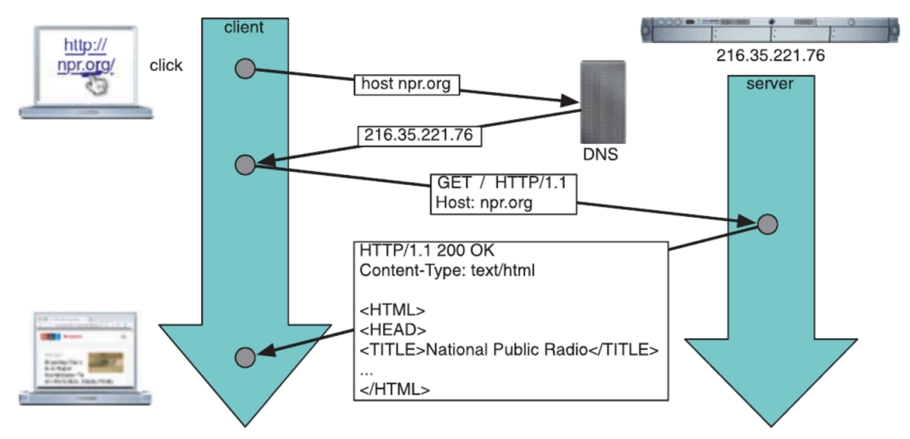
The three key ingredients of the Web:
URLs: Uniform Resource Locators, page addresses to link to pages
HTML: HyperText Markup Language to write web pages
HTTP: HyperText transfer Protocol for web clients and servers to communicate
In the early 1990s, Tim Berners-Lee introduced an effective directed hyperlink model
This paradigm of hypertext language, along with his communication protocol for Web browsers and servers, became very popular, and the Web was born.
Each page has a URL (Uniform Resource Locator) which can be linked by other pages
In The 1990’s the Web was still mainly a network in which content creators were distinct from its consumers (required special skills to make content)
Web-2.0: consumers became creators (text, videos, photos, etc)
Web-logs (blogs) became the fastest-growing segment of the Web.
Content storage is still centralized by large companies
Youtube, Social media cites: Friendster, Orkut, MySpace, LinkedIn, and Facebook.
Web 3.0: An idea for a new iteration of the Web emerged in 2014, which incorporates decentralization, blockchain technologies, and token-based economics
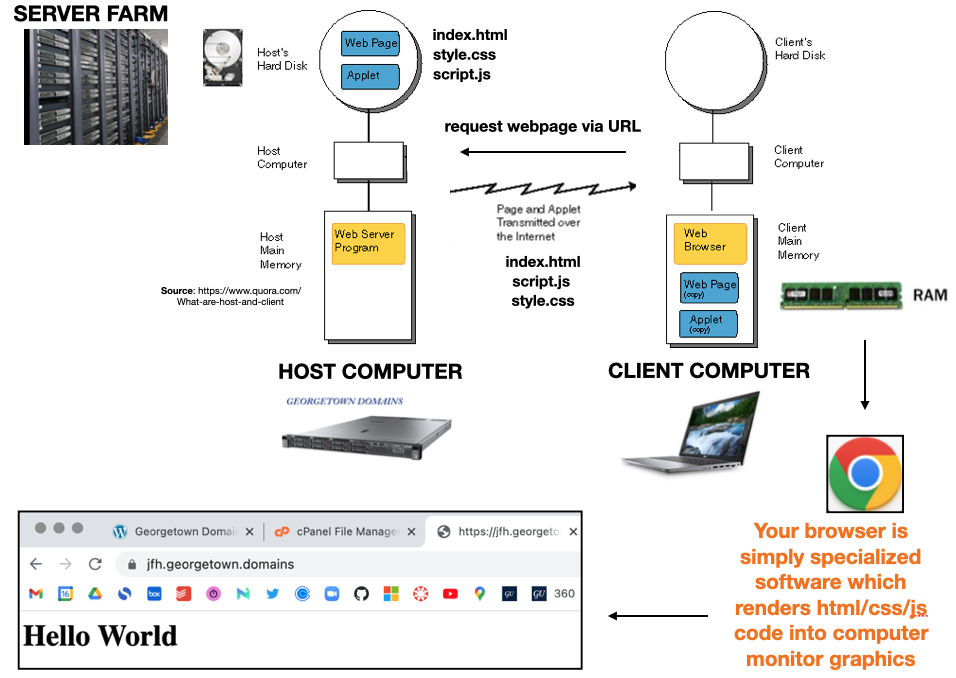
The server is the computer where the content “lives” on hard-drive
Any program using the HTTP protocol to request content from Web servers is a client.
The browser is specialized software for rendering HTML,CSS,JS content.
Web Crawlers
Information on the Web is always changing and scattered across billions of pages served by millions of servers around the globe
Web crawlers are programs that automatically download Web pages, to collect information that can be analyzed and mined in a central location.
The primary application of crawlers are search engines
A search engine takes the information collected by a crawler and creates an index
The index maps content (keywords and phrases) to the pages, for rapid retrieval
Search engine also rank results, to provide high quality results.
Other applications: business intelligence, digital libraries, webometrics tools, research
Malicious applications: harvesting email addresses and personal information for spam, phishing, and identity theft
How web crawlers work
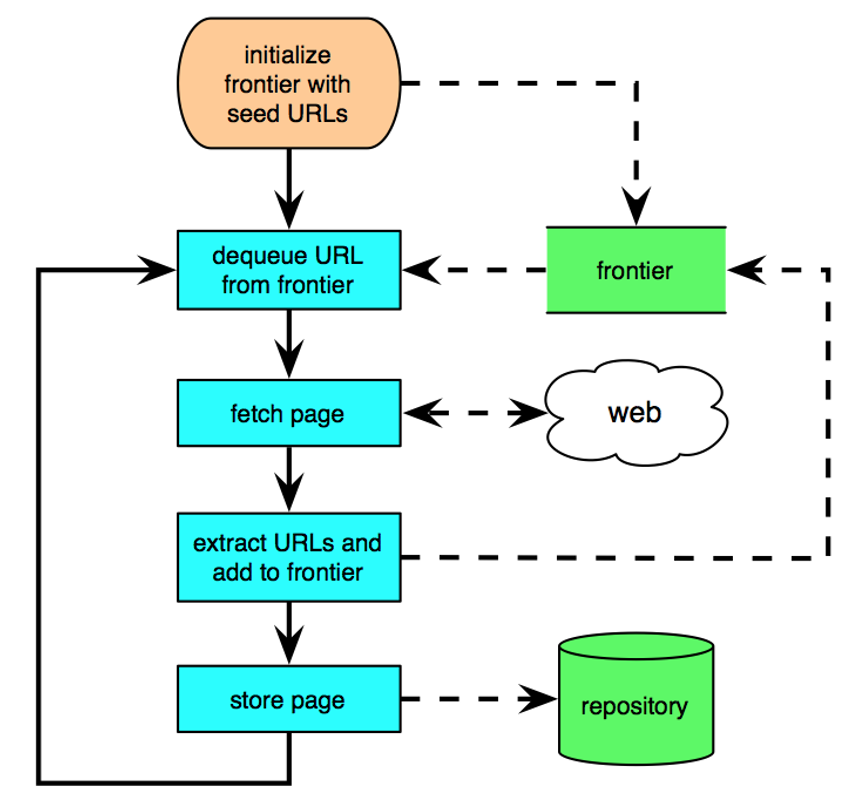
The basic concept of a crawler is simple: a breadth-first traversal of the Web graph, as in the BFS algorithm
Start from a set of high-quality seed pages, recursively extracts the links within them to fetch more pages
The queue of unvisited URLs (frontier)
Fetch pages dequeued from the frontier, extract links and add them to the frontier
Stores the page (and other extracted info, i.e index terms) in a repository.
Devil in the details: complications due to scalability, page revisit scheduling, spider traps, canonical URLs, robust HTML parsing, and the server ethics
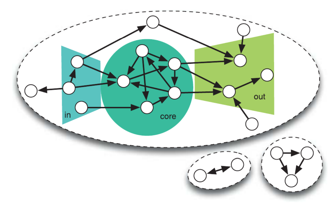
Large-scale web-crawls reveal the structure of the web with various (weakly) connected components.
Their sizes tend to have a skewed distribution, with the largest “giant component” dominating (with more than 90% of all pages) and a great many small ones.
The bow-tie structure of the Web graph. Components are highlighted by dashed ovals. The giant component has a giant strongly connected component (sometimes referred to as the “core”), an in-component (“in”), and an out-component (“out”).
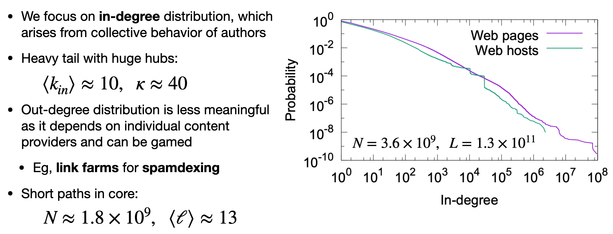
Web degree distributions
Note how the plot suggests the presence of a power law
Network topical locality
Web links are not random!
Overview
Recall Homophily: The tendency of similar nodes to be connected (Birds of a feather flock together)
Nodes in information networks, such as Web pages, Wikipedia articles, and research papers tend to exhibit Homophily
e.g. two pages about sports are typically more similar than a page about sports and one about music.
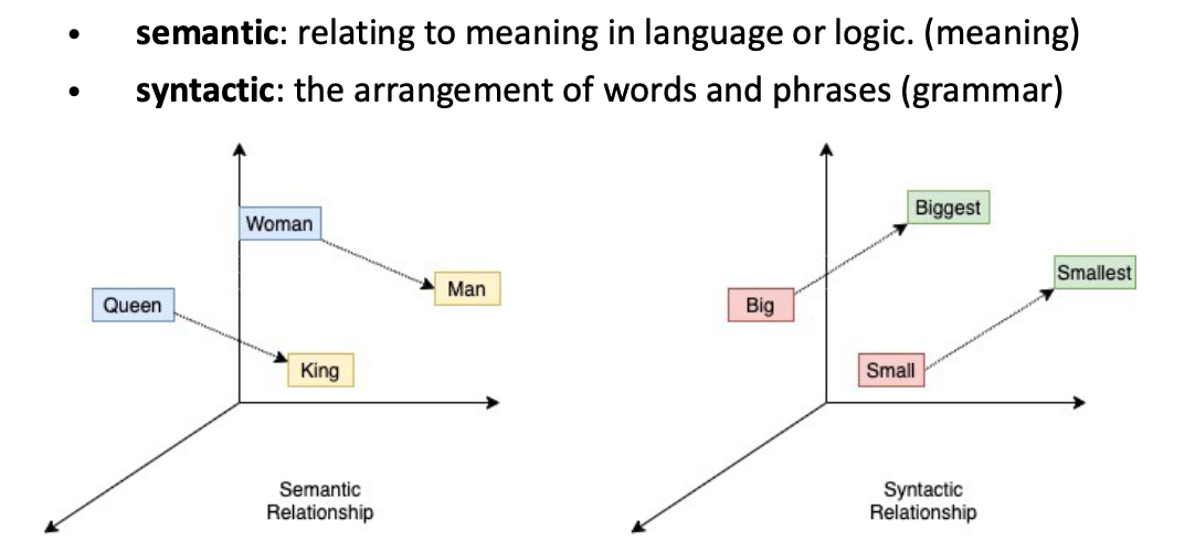
In this case, links encode semantic information about the nodes.
Two pages about related topics may link to each other or may have a short path connecting them.
When this happens we say that the network has topical locality.
The reason the effect emerges is intuitive: when new pages are created, the authors want to help readers by linking to topically relevant information.
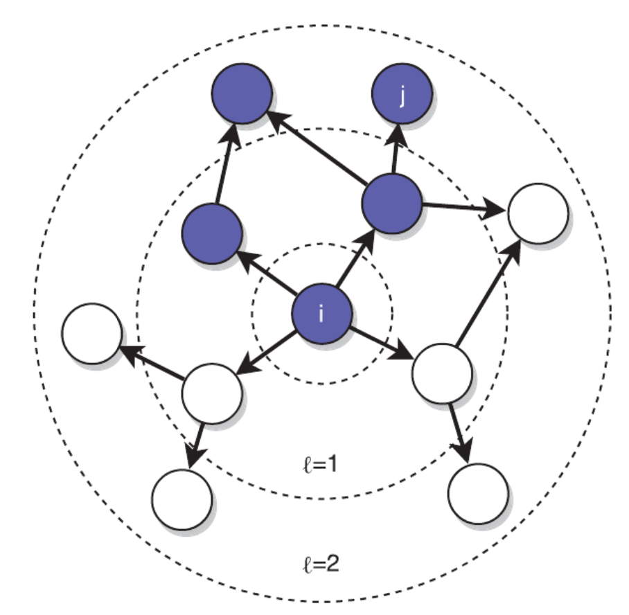
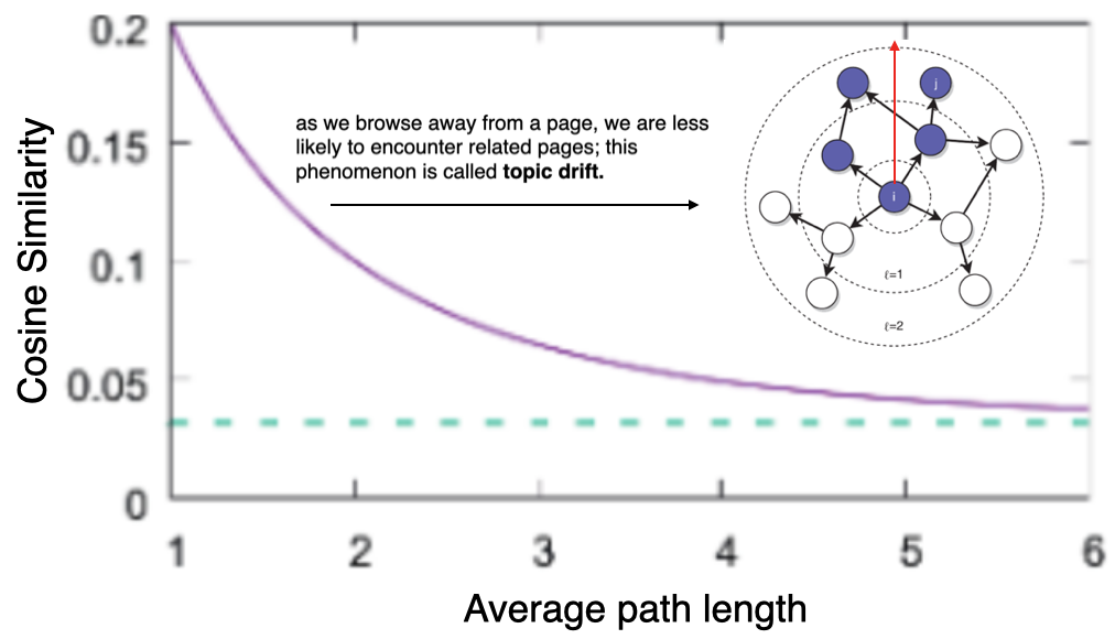
One way to quantify topical locality is to measure how likely a target page, within a given distance from a source, is related to the source’s topic.
e.g. In this network, half of the pages at distance \(\ell=1\) from page \(i\), and one-third of the pages at distance \(\ell=2\), are about the same topic (shown in blue).
Topical locality makes Web browsing possible as we stay on topic
Crawlers use BFS because of topical locality, to target good-quality pages linked by other good-quality pages
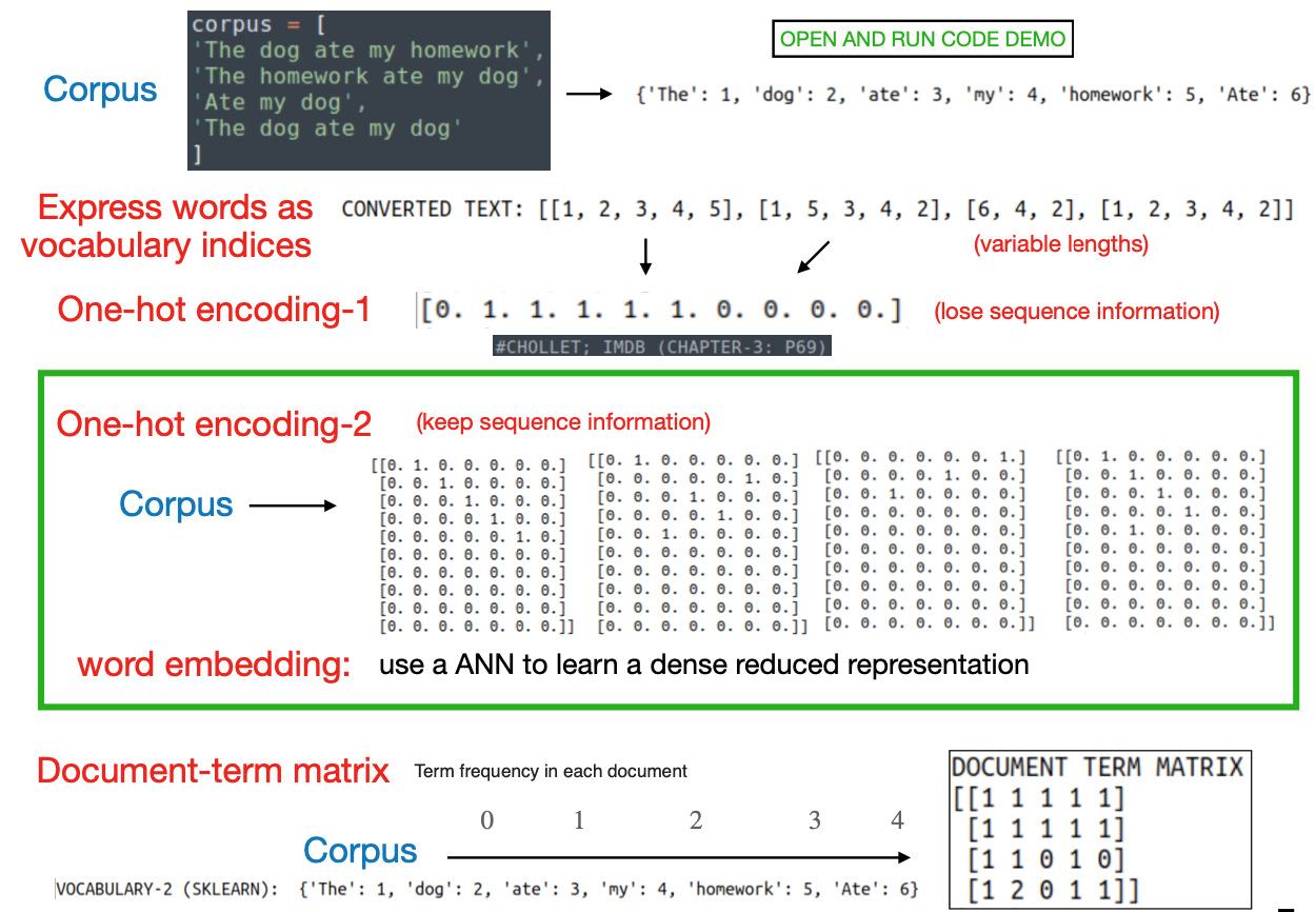
Vectorization: Process of transforming text into numeric tensors
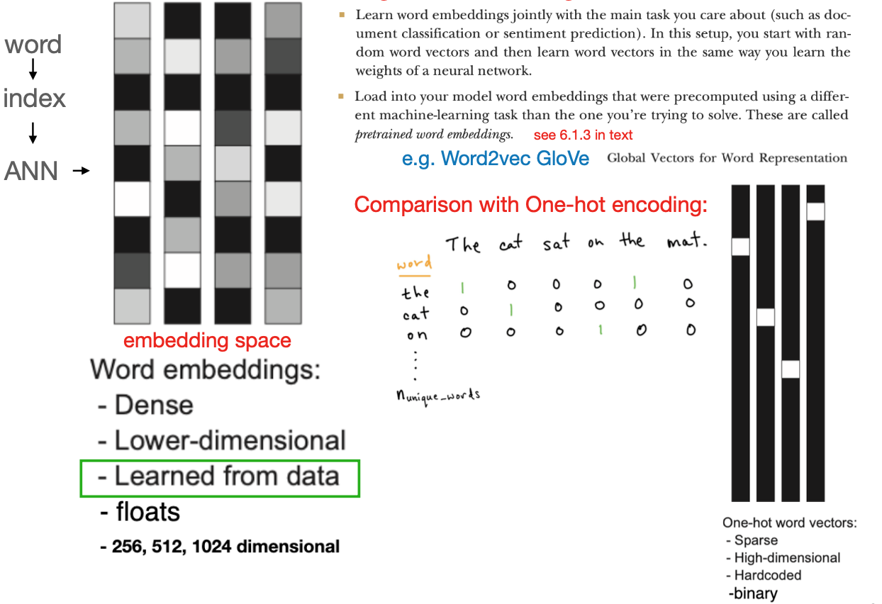
Word embeddings
Cosine similarity: Closer look
Often we need to measure the similarity between two documents, Web pages, blurbs of text, or tag cloud, etc.
Let us represent each document \(d\) as a high-dimensionality vector, with a dimension associated with each term in the vocabulary: \(\vec{d}=\left\{w_{d, 1}, \ldots, w_{d n_1}\right\}\), where \(w_{d, t}\) is the weight of term \(t\) in \(d\), and \(n_t\) is the total number of terms.
There are various ways to calculate the weights. Typically they are proportional to the frequency with which a term appears in a document
One often removes “noise words” (stop-words) that are not meaningful
It is also common to discount the weights of terms that occur in many documents, as they have low discriminating power.
Then we can compute the similarity between two documents \(d_1\) and \(d_2\) by measuring the cosine between their vectors: \[\cos \left(\vec{d}_1, \vec{d}_2\right)=\frac{\vec{d}_1}{\left\|\vec{d}_1\right\|} \cdot \frac{\vec{d}_2}{\left\|\vec{d}_2\right\|}=\frac{\sum_t w_{d_1, t} w_{d_2, t}}{\sqrt{\sum_t w_{d_1, t}^2} \sqrt{\sum_t w_{d_2, t}^2}}\] If the terms in \(d_1\) are also present in \(d_2\) and vice versa, the cosine is close to one; if the two documents do not share any terms, the cosine is zero. Note that the cosine is normalized by the norm, or size of each vector: \[
\|\vec{d}\|=\sqrt{\sum_t w_{d, t}^2}
\] This way, a longer document will not appear to be similar to many others just because it has many terms: its large norm would decrease the similarity.
Web topical locality, measured by breadth-first search crawls from 100 sets of seed pages for many topics.
For each crawl, we report the average cosine similarity between seeds and pages as a function of the average path length between them.
Notice the strong topical locality: the similarity between seeds and pages one link away is more than six times higher than the noise level between random pages (dashed line).
Topic drift is illustrated by the decay in average similarity between seed and crawled pages, toward the noise level.
 Source: DOI:10.1017/9781108653947