fig, ax = plt.subplots(figsize=(5, 3.0))
draw_graph(G, pos, ax, title="Toy graph: triangle {0,1,2} + pendant node 3")
plt.show()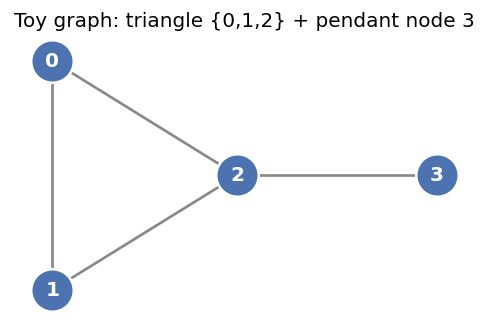
Background review
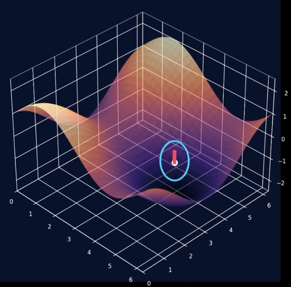
In multivariable calculus, the two fundamental types of functions are:
Here are the main differential operators that act on these fields:
A scalar operator that takes a scalar field \(f(x_1,\dots,x_n)\) and reports, at each point, how much \(f\) differs from the average of its immediate surroundings.
\[\Delta f \;=\; \nabla\cdot\nabla f \;=\; \sum_{i=1}^{n}\frac{\partial^2 f}{\partial x_i^2} \;=\; \operatorname{tr}(\operatorname{Hess} f).\]
Reading the notation: \(\nabla\) is the gradient (a vector of first derivatives). Apply it twice, taking the divergence of the gradient, and the dot product collapses the vector back to a scalar, hence the “squared” in \(\nabla^2\). Three readings of the same object:
Sign: \(\Delta f > 0\) at a dip (center sits below its neighbors), \(\Delta f < 0\) at a bump, \(\Delta f = 0\) when \(f\) already equals its local average (harmonic).
In 3D Cartesian coordinates \((x, y, z)\) this is just the three unmixed second derivatives:
\[\nabla^2 f \;=\; \frac{\partial^2 f}{\partial x^2} + \frac{\partial^2 f}{\partial y^2} + \frac{\partial^2 f}{\partial z^2}.\]
In networks, discretize it and swap “tiny sphere” for “wired neighbors,” and \(\Delta\) becomes the graph Laplacian.
Source: https://youtu.be/7ZmRqSeoylU?si=SKGiAa0eEAhCyVUv
\[\text { rate of change of } u=\kappa \text { (neighborhood average of } u-u \text { at the point). }\]
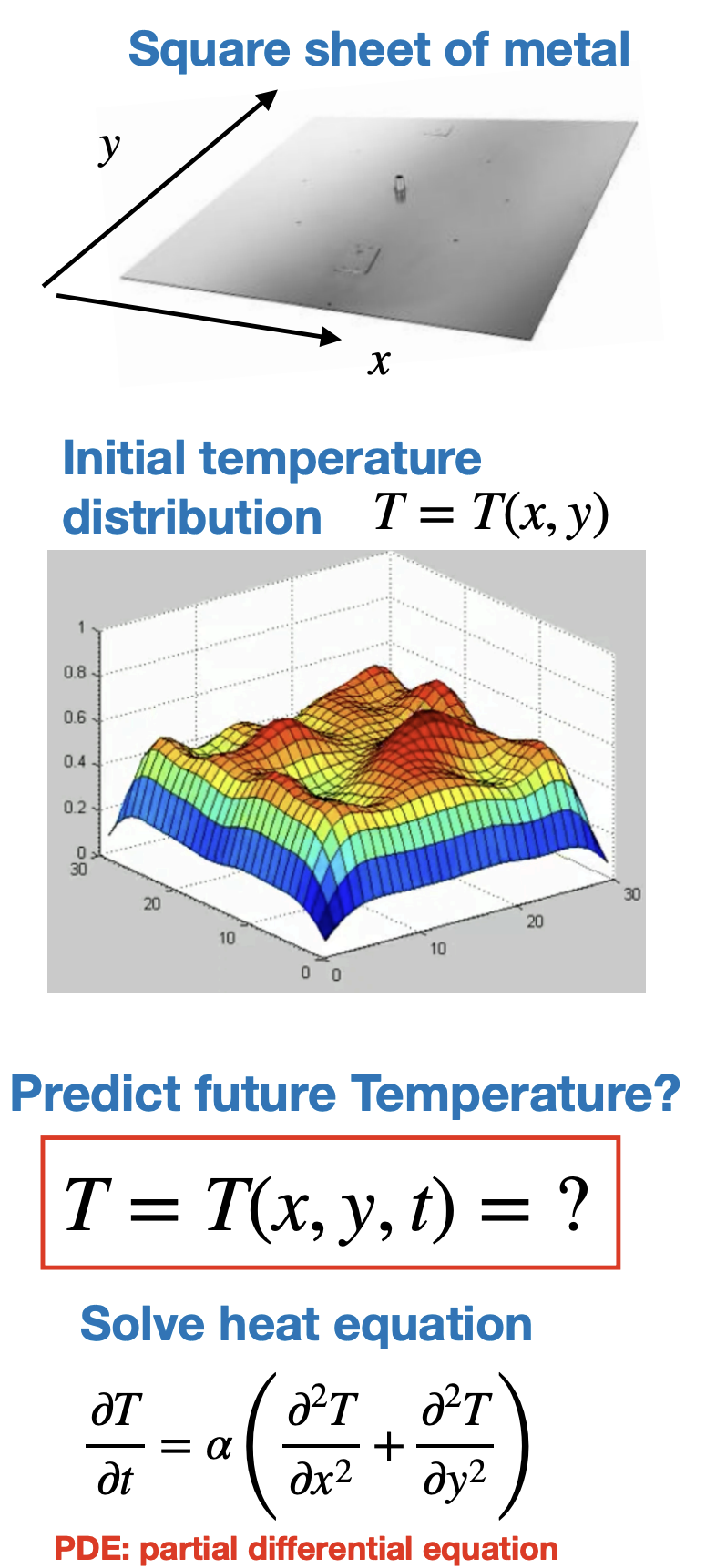
\[ \frac{\partial u}{\partial t} \;=\; \alpha\left(\frac{\partial^2 u}{\partial x^2} + \frac{\partial^2 u}{\partial y^2}\right) \;=\; \alpha\,\nabla^2 u. \]
To solve it you also need: - Initial: the starting temperature \(u(x, y, 0) = u_0(x, y)\) (say, a hot spot). - Boundary: edges held fixed (Dirichlet), insulated (Neumann), or losing heat to air (Robin).
Mesh the sheet into a grid of nodes and \(\alpha\nabla^2 u\) becomes \(-\alpha L u\): the graph diffusion from the deck.
Analytic (separation of variables). Split \(u(x,t) = X(x)\,T(t)\), and the PDE breaks into two ODEs. The spatial part forces \(X\) to be an eigenfunction of \(\nabla^2\) (a sine/cosine mode set by the boundaries), and each mode decays in time at its own rate:
\[u(x,t) = \sum_k c_k\,\underbrace{\phi_k(x)}_{\text{spatial mode}}\;\underbrace{e^{-\alpha\lambda_k t}}_{\text{decay}}.\]
Numerical (finite differences). Chop space into a grid and replace \(\nabla^2\) with the neighbor stencil, which is exactly \(-L\) on the grid graph. Then step time forward:
\[u^{n+1} = u^{n} + \alpha\,\Delta t\,(-L\,u^{n}).\]
Same skeleton. The analytic modes \(\phi_k\) are eigenvectors of the continuous \(\nabla^2\); the numerical update runs on eigenvectors of the discrete \(L\). Both say: decompose into modes, let each decay.
For an undirected, unweighted graph with adjacency matrix \(A\) and degree matrix
Concepts generalize to weighted graphs with \(A\) and \(D\) replaced by \(W\) and \(D\)
For an undirected, unweighted graph with adjacency matrix \(A\) and degree matrix \(D = \operatorname{diag}(k_1, \dots, k_N)\) (degrees on the diagonal, zeros elsewhere):
\[L = D - A\]
We will build it on this 4-node toy graph: a triangle \(\{0,1,2\}\) with a pendant node \(3\).
fig, ax = plt.subplots(figsize=(5, 3.0))
draw_graph(G, pos, ax, title="Toy graph: triangle {0,1,2} + pendant node 3")
plt.show()
Read the degrees straight off the picture: \(k_0 = 2,\ k_1 = 2,\ k_2 = 3,\ k_3 = 1\).
\[ A=\begin{pmatrix}0&1&1&0\\1&0&1&0\\1&1&0&1\\0&0&1&0\end{pmatrix},\quad D=\begin{pmatrix}2&0&0&0\\0&2&0&0\\0&0&3&0\\0&0&0&1\end{pmatrix},\quad L=D-A=\begin{pmatrix}2&-1&-1&0\\-1&2&-1&0\\-1&-1&3&-1\\0&0&-1&1\end{pmatrix} \]
Notice every row of \(L\) sums to zero. That single fact drives much of what follows.
nodelist = [0, 1, 2, 3]
A = nx.to_numpy_array(G, nodelist=nodelist)
D = np.diag(A.sum(axis=1))
L = D - A

def show(M, name):
    print(f"{name} =")
    print(pd.DataFrame(M.astype(int), index=nodelist, columns=nodelist).to_string())
    print()

show(A, "A"); show(D, "D"); show(L, "L")
print("Row sums of L:", L.sum(axis=1).astype(int))   # all zero

fig, ax = plt.subplots(figsize=(4.0, 3.4))
im = ax.imshow(L, cmap="coolwarm", vmin=-3, vmax=3)
ax.set_xticks(range(4)); ax.set_yticks(range(4))
ax.set_xticklabels(nodelist); ax.set_yticklabels(nodelist)
for i in range(4):
    for j in range(4):
        ax.text(j, i, int(L[i, j]), ha="center", va="center",
                color="white" if abs(L[i, j]) > 1.5 else "black", fontweight="bold")
ax.set_title("L = D - A")
plt.colorbar(im, ax=ax, fraction=0.046, pad=0.04)
plt.show()
A =
0 1 2 3
0 0 1 1 0
1 1 0 1 0
2 1 1 0 1
3 0 0 1 0
D =
0 1 2 3
0 2 0 0 0
1 0 2 0 0
2 0 0 3 0
3 0 0 0 1
L =
0 1 2 3
0 2 -1 -1 0
1 -1 2 -1 0
2 -1 -1 3 -1
3 0 0 -1 1
Row sums of L: [0 0 0 0]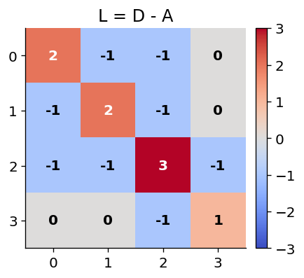
For a smooth function \(f(x)\),
\[ \nabla^2 f = \frac{\partial^2 f}{\partial x^2} + \frac{\partial^2 f}{\partial y^2} +\cdots \]
The graph Laplacian is the discrete version of the continuous Laplacian, it measures how much a node differs from its local neighborhood, just as the continuous Laplacian measures how a function differs from its local surroundings.
For a graph, the analogous quantity is
\[ (L\mathbf{x})_i = \sum_{j\in N(i)} (x_i-x_j), \]
where
\[ L = D - A. \]
The graph Laplacian \(L\) is an operator that maps a node signal \(x\) to the vector of local deviations, \((L x)_i=\sum_{j \sim i}\left(x_i-x_j\right)\), measuring how far each node’s value departs from its neighbors’.
| Continuous Domain | Graph Domain |
|---|---|
| Space | Network |
| Nearby points | Neighboring nodes |
| Second derivative | Neighbor differences |
| \(\nabla^2\) | \(L=D-A\) |
\[\boxed{(L x)_i=\sum_{j \in N(i)}\left(x_i-x_j\right)}\]
Graph: \(0-1-2\) (a path).
Signal: \(x=[0,4,0]\), so node 1 is a spike sitting above two flat neighbors.
Note: We can think of this square matrix as a linear operator that transforms a node-level vectors \(x\)
Apply the operator node by node using \((L x)_i=\sum_{j \in N(i)}\left(x_i-x_j\right)\) :
\[ L x=[-4,+8,-4] . \]
The adjacency \(A\) records who is wired to whom (the neighbor sets \(N(i)\) ), and the degree \(D\) is just its row sums on the diagonal:
\[ A=\left(\begin{array}{ccc} 0 & 1 & 0 \\ 1 & 0 & 1 \\ 0 & 1 & 0 \end{array}\right), \quad D=\left(\begin{array}{ccc} 1 & 0 & 0 \\ 0 & 2 & 0 \\ 0 & 0 & 1 \end{array}\right), \quad L=D-A=\left(\begin{array}{ccc} 1 & -1 & 0 \\ -1 & 2 & -1 \\ 0 & -1 & 1 \end{array}\right) . \]
Confirm with the matrix:
\[ L\left(\begin{array}{l} 0 \\ 4 \\ 0 \end{array}\right)=\left(\begin{array}{c} 1(0)-1(4)+0 \\ -1(0)+2(4)-1(0) \\ 0-1(4)+1(0) \end{array}\right)=\left(\begin{array}{c} -4 \\ 8 \\ -4 \end{array}\right) \]
A symmetric matrix \(M\) is positive semi-definite (PSD) when
\[x^{T} M x \ge 0 \quad \text{for every vector } x.\]
\[0 = \lambda_1 \le \lambda_2 \le \dots \le \lambda_N.\]
\[(L x)_i=\sum_{j \in N(i)}\left(x_i-x_j\right)\]
Weight each node’s deviation by its own value \(x_i\) and sum over all nodes:
\[x^{T} L x = \sum_i x_i\,(Lx)_i = \sum_i x_i \sum_{j \in N(i)}(x_i - x_j).\]
Every undirected edge \(\{i,j\}\) shows up twice, once from each endpoint. Add the pair:
\[x_i(x_i - x_j) + x_j(x_j - x_i) = (x_i - x_j)^2.\]
So the double sum collapses to one square per edge:
\[\boxed{\,x^{T} L x = \sum_{(i,j)\in E}(x_i - x_j)^2 \;\ge\; 0\,}\]
Example (\(x = [0,4,0]\) on the path, \(Lx = [-4, 8, -4]\)):
\[x^{T} L x = 0(-4) + 4(8) + 0(-4) = 32 = \underbrace{(0-4)^2}_{\text{edge }0\text{-}1} + \underbrace{(4-0)^2}_{\text{edge }1\text{-}2} = 32.\]
The operator \(L x\) reports per-node deviation;
the scalar \(x^{T} L x\) aggregates it into total disagreement across edges (the Dirichlet energy).
The central identity:
\[x^{T} L x = \sum_{(i,j)\in E} A_{ij}\,(x_i - x_j)^2.\]
The same quantity \(x^{T} L x\) is the Dirichlet energy of the signal \(x\).
Compare a smooth signal against a rough one on the toy graph.
x_smooth = np.array([0.9, 1.0, 0.2, 0.0])   # similar on the triangle, decays on the pendant
x_rough  = np.array([1.0, 0.0, 1.0, 0.0])   # alternates, disagrees on most edges

for name, v in [("smooth", x_smooth), ("rough ", x_rough)]:
    print(f"{name} x = {v}   ->   Dirichlet energy  x^T L x = {v @ L @ v:.2f}")
smooth x = [0.9 1. 0.2 0. ] -> Dirichlet energy x^T L x = 1.18
rough x = [1. 0. 1. 0.] -> Dirichlet energy x^T L x = 3.00Because every row of \(L\) sums to zero,
\[L\mathbf{1} = \mathbf{0}, \qquad \mathbf{1} = [1, 1, \dots, 1]^{T}.\]
So \(\mathbf{1}\) is an eigenvector with eigenvalue \(0\), and the smallest eigenvalue is always exactly zero.
ones  = np.ones(4)
evals = np.linalg.eigvalsh(L)
print("L @ 1            =", (L @ ones).astype(int))     # the zero vector
print("eigenvalues of L =", np.round(evals, 3))         # smallest is exactly 0
L @ 1 = [0 0 0 0]
eigenvalues of L = [0. 1. 3. 4.]A sharper statement:
the number of zero eigenvalues equals the number of connected components.
Edge case: two disjoint triangles, no bridge between them.
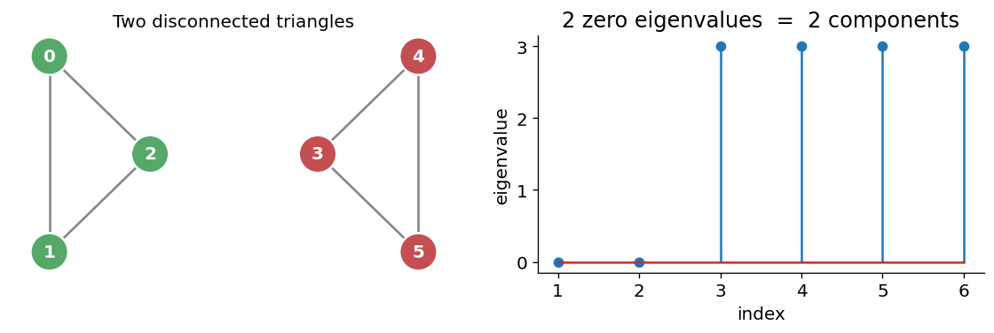
eigenvalues: [-0. -0. 3. 3. 3. 3.]The second smallest eigenvalue \(\lambda_2\) is the algebraic connectivity, or Fiedler value. It grades how well-connected and how robust the graph is.
So \(\lambda_2\) lives in \([0, N]\). Let us see all three regimes on \(N = 6\) nodes.
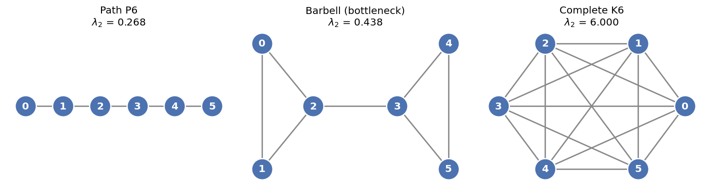
N = 6 for all three.  lambda_2 runs from ~0 up to N.
Path P6   : lambda_2 = 0.268
Barbell   : lambda_2 = 0.438
Complete  : lambda_2 = 6.000   (= N = 6, only K_N reaches this)
The eigenvector belonging to \(\lambda_2\) is the Fiedler vector. It assigns each node a real number.
Spectral bisection: split nodes by the sign of their Fiedler value. The split lands across the bottleneck, cutting as few edges as possible.
On the barbell, this separates the two triangles and cuts only the single bridge.
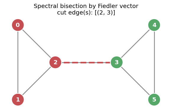
Fiedler vector: [-0.465 -0.465 -0.261  0.261  0.465  0.465]
sign split : [1 1 1 0 0 0] (0 = green group, 1 = red group)Almost nothing changes.
\[x^{T} L x = \sum_{(i,j)\in E} A_{ij}\,(x_i - x_j)^2.\]
The graph Laplacian is an important graph-level matrix similar to the adjacency matrix.
For an undirected, unweighted graph with adjacency matrix \(A\) and degree matrix \(D= \operatorname{diag}\left(k_1, \ldots, k_N\right)\) (node degree along the main diagonal an zero everywhere else), the graph Laplacian is \[ L=D-A \]
It is important because it is another well behaved, mathematically, well structured square matrix that describes the graph
One of the major reasons that it is important is that it is a positive semi-definite matrix which has several important properties in linear algebra.
Recall the definition of a positive semi-definite matrix.
A positive semi-definite matrix acts like a multi-dimensional “non-negative number,” meaning that when you use it to transform any vector, the resulting vector never points in the opposite direction of the original (the angle between them is always less than or equal to \(90^\circ\))
Mathematically, a symmetric matrix \(M\) is positive semi-definite if for every non-zero vector \(x\), the quadratic form is non-negative: \(x^T M x \ge 0\)
Motivation: Where it emerges in network science
Important properties: From a linear algebra perspective, the graph Laplacian matrix (\(L = D - A\)) possesses several elegant structural properties that make it a powerful tool for analysis:
Symmetry: For any undirected graph with real weights, \(L\) is a symmetric matrix (\(L = L^T\)). This guarantees that all of its eigenvalues are real numbers and its eigenvectors are orthogonal.
Positive Semi-Definiteness: The Laplacian is a positive semi-definite matrix (\(x^T L x \ge 0\) for any vector \(x\)). Consequently, all of its eigenvalues are non-negative (\(0 = \lambda_1 \le \lambda_2 \le \dots \le \lambda_n\)).
Trivial Smallest Eigenvalue: The smallest eigenvalue is always exactly zero (\(\lambda_1 = 0\)). Its corresponding eigenvector is the all-ones vector (\(\mathbf{1} = [1, 1, \dots, 1]^T\)), because each row of \(L\) sums to zero.
Multiplicity of Zero Indicates Components: The multiplicity of the eigenvalue \(0\) equals the exact number of connected components in the graph. For a fully connected graph, there is exactly one zero eigenvalue.
Diagonally Dominant: \(L\) is a diagonally dominant matrix because the diagonal entry for any node \(i\) (its degree, \(D_{ii}\)) is exactly equal to the sum of the absolute values of the off-diagonal entries in that row (\(\sum_{j \neq i} |A_{ij}|\)).
Quadratic form: The quadratic form of the graph Laplacian \(L\) for a node state vector \(x \in \mathbb{R}^n\) is \(x^T L x\)
This can be written in two ways, depending on how the sum is constructed \(\quad x^T L x=\frac{1}{2} \sum_{i, j} A_{i j}\left(x_i-x_j\right)^2=\sum_{(i, j) \in E} A_{i j}\left(x_i-x_j\right)^2\) (where the 1/2 handles double counting in the summation)
Graph Dirichlet Energy: It quantifies the global smoothness of a graph signal \(x\). A low value indicates homophily, where structurally adjacent nodes share highly correlated states.
Spectral Clustering Objective: Minimizing this quadratic form under the constraint \(x \perp \mathbf{1}\) directly solves the relaxed RatioCut problem, partitioning the network into communities while minimizing inter-cluster edge cuts.
Weighted case
Directed Case: For directed graphs there is no single canonical Laplacian, because \(A\) is asymmetric and the clean spectral theory above relies on symmetry.