ODE Numerical methods
Initial value problems
Source: https://cdn.mathpix.com/snip/images/-ud5z7_akoNrXkb2rUt6s5cnaC4rbpAbaxJBWDF0YmA.original.fullsize.png
Definitions
- An ordinary differential equation (ODE) is one where derivatives of an unknown function of one variable appear.
- The order of a differential equation is the highest derivative that appears in it.
- An equation can be first-order, second-order, …
Standard form for ODE initial value problems (IVPs)
- First-order: \(y^{\prime}(t)=f(t, y(t))\) and \(y\left(t=t_0\right)=y_0\) where \(t_0, y_0\) are known values, \(f\) is a known function, and \(y(t)\) is an unknown function
- Second-order: \(y^{\prime \prime}(t)=f\left(t, y(t), y^{\prime}(t)\right)\) and \(y\left(t=t_0\right)=y_0\) and \(y^{\prime}\left(t=t_0\right)=\mathrm{dy}_0\)
- Etc. for higher order; in general, an ODE of order \(n\) can be written as
\[ \frac{d^n y}{d t^n}=f\left(t, y, \frac{d y}{d t}, \frac{d^2 y}{d t^2}, \ldots, \frac{d^{n-1} y}{d t^{n-1}}\right) \]
- the corresponding initial values as
\[ y\left(t_0\right)=y_0^{(0)}, \frac{d y}{d t}\left(t_0\right)=y_0^{(1)}, \frac{d^2 y}{d t^2}\left(t_0\right)=y_0^{(2)}, \ldots, \frac{d^{n-1} y}{d t^{n-1}}\left(t_0\right)=y_0^{(n-1} \]
- all \(n\) initial values must be given at the same \(t=t_0\)
Some examples of ODEs
First-order: - Cooling of something hot - Epidemic spread (e.g. the susceptible-recovered-infected [SIR] model) Second-order - Mechanics (Newton’s Second Law), electromagnetism - Waves, vibrations (e.g. shear-building model)
Fourth-order - Beam deflection (Euler-Bernoulli theory)
A typical first-order ODE initial-value problem
- Given the ODE \(y^{\prime}(t)=f(t, y(t))\), and knowing that \(y(a)=y_0\) (the initial value; the initial point is denoted \(a\) or \(t_0\) ), find \(y(b)\) (where \(b\) is some other point).
- Or sometimes we may want to find \(y\) at various points between \(a\) and \(b\), not just at the one point \(b\)
- Example: If \(y^{\prime}(t)=t-y\) and \(y(t=0)=1\), estimate \(y(t=2)\).
- So \(a=0, b=2, y_0=1\)
- Some ODEs can be solved analytically (cf. your differential equations class). Here, we will concentrate on numerical methods that enable us to find approximate solutions even where there is no analytic solution.
Aside: Integrating factor
You can use the integrating factor method for first-order linear ODEs of the form:
\(\frac{dy}{dt} + p(t)y = q(t)\)
It applies when:
- The equation is linear in \(y\)
- Coefficients \(p(t)\) and \(q(t)\) are known functions of \(t\)
The integrating factor is \(\mu(t) = e^{\int p(t)\,dt}\), which allows the left-hand side to be written as a product rule derivative.
Aside: Analytic solution
Solve the ODE:
\(y'(t) = t - y, \quad y(0) = 1\)
Step 1: Standard linear form:
\(y' + y = t\)
Step 2: Integrating factor:
\(\mu(t) = e^t\)
Step 3: Multiply both sides:
\(e^t y' + e^t y = t e^t \Rightarrow \frac{d}{dt}(e^t y) = t e^t\)
Step 4: Integrate:
\(e^t y = \int t e^t dt = t e^t - e^t + C\)
Step 5: Solve:
\(y(t) = t - 1 + C e^{-t}\)
Step 6: Apply initial condition \(y(0) = 1\):
\(1 = -1 + C \Rightarrow C = 2\)
Final solution:
\(\boxed{y(t) = t - 1 + 2e^{-t}}\)
\(y(2)=2-1+2e^{-2}\approx 1.2706705\)
Numerical Solving by steps
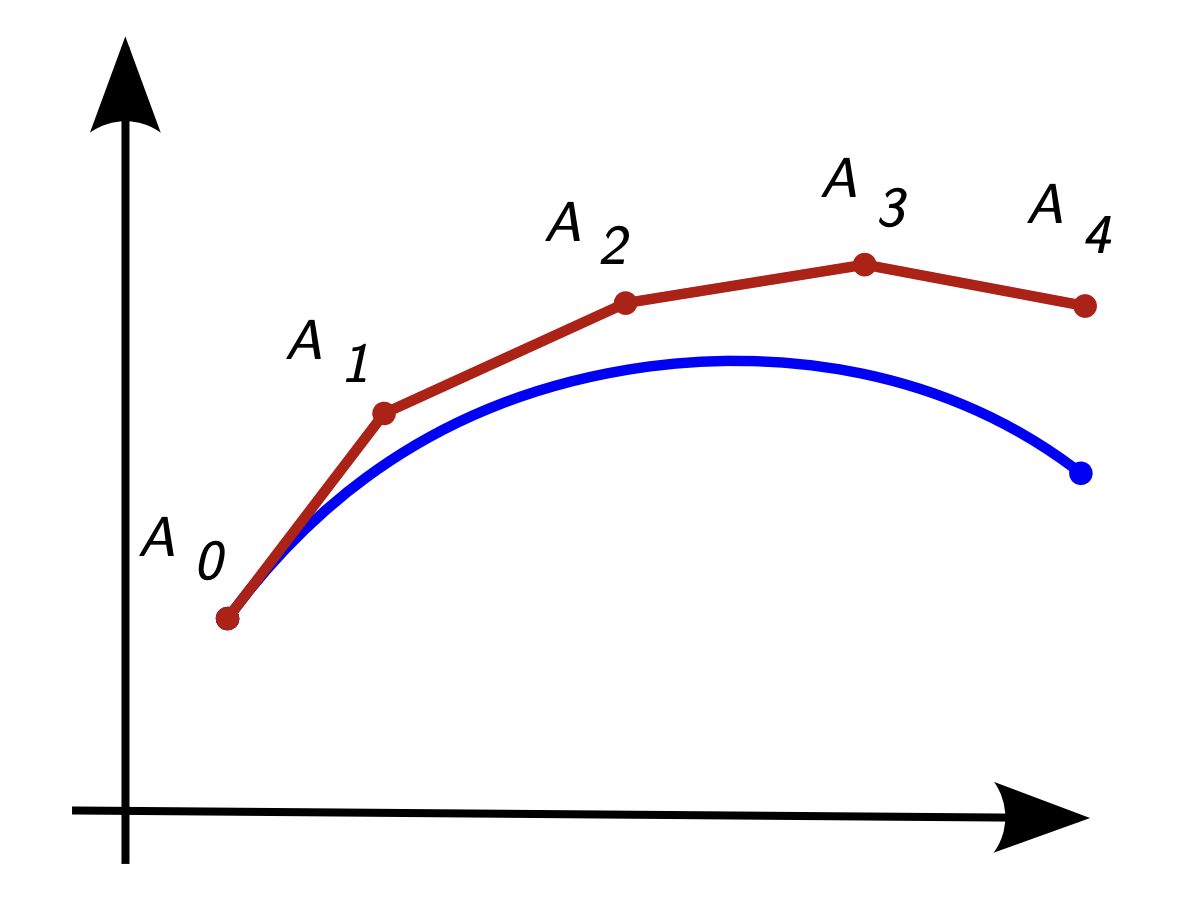
- Typically, we divide the interval \([a, b]\) into segments by taking points (often equally spaced) \(a=t_0, t_1, t_2, \ldots t_N=b\) and apply a numerical solution procedure to each segment starting with the initial point
- Thus, we would start with \(t_0\), where we know that the value of \(y\) is \(y_0\). Then we would estimate the value of \(y\) at \(t_1\) as \(y_1\).
- We use this estimated \(y_1\) as the new initial value to estimate \(y\) at \(t_2\), calling this estimate \(y_2\)
- And continue until, after \(N\) steps, we get \(y_N\), which is the estimated value of \(y\) at \(t=b\)
- Generally, for a given numerical method applied at each step, the smaller each step is, the more accurate our estimate of \(y(b)\)
Euler’s Method for Solving ODEs
Goal: Approximate the solution to an initial value problem: \[ \frac{d y}{d t}=f(t, y), \quad y\left(t_0\right)=y_0 \]
Intuition - We don’t know the exact curve \(y(t)\), but we know the slope at any point: \(f(t, y)\) - Use the slope at the current point to take a small step forward:
\[ y_{n+1} \approx y_n+h \cdot f\left(t_n, y_n\right) \]
- This is like tangent line approximation:
\[ y(t+h) \approx y(t)+h \cdot y^{\prime}(t) \]
Euler’s Update Rule Given step size \(h\), starting at \(\left(t_0, y_0\right)\) :
\[ \begin{aligned} & t_{n+1}=t_n+h \\ & y_{n+1}=y_n+h \cdot f\left(t_n, y_n\right) \end{aligned} \]
Repeat for \(n=0,1,2, \ldots\)
Euler’s method: Example
- As we saw before, for this numerical method, each step is \(y_{i+1}=y_i+h f\left(t_i, y_i\right)\), where \(h\) is the step size \(\left(t_{i+1}-t_i\right)\).
- For our example case, if we take \(N=3\) equal steps so that \(h\) is \(\frac{b-a}{N}=\frac{2}{3}\),
- \(y_1=y_0+h\left(t_0-y_0\right)=\frac{1}{3}\)
- \(y_2=y_1+h\left(t_1-y_1\right)=\frac{5}{9}\)
- \(y_3=y_2+h\left(t_2-y_2\right)=\frac{29}{27} \approx 1.074\), which is the obtained estimate for \(y(t=2)\).
Sketch of several Euler method steps
Alternative methods: Heun’s method
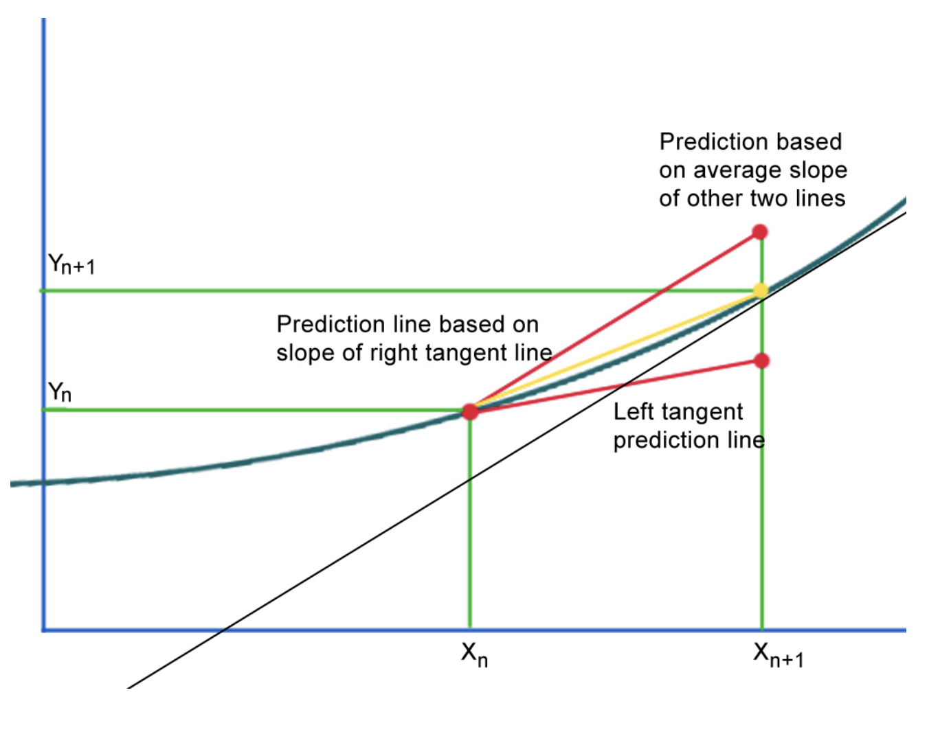
This is more elaborate, in that at each step there are two estimates of the average value of \(f\) between \(t_i\) and \(t_{i+1}\), which are averaged to estimate how much \(y\) changes over the step: \(y_{i+1}=y_i+\frac{1}{2}\left(K_1+K_2\right)\), where - \(K_1=h f\left(t_i, y_i\right)\) - \(K_2=h f\left(t_i+h, y_i+K_1\right)\)
For our example case, with \(N=3\) equal steps as before, - First step: \(K_1=h\left(t_0-y_0\right)=-\frac{2}{3}, K_2=h\left(t_1-\left(y_0+K_1\right)\right)=\) \(\frac{2}{9}, y_1=y_0+\frac{1}{2}\left(K_1+K_2\right)=\frac{7}{9}\) - Second step: \(K_1=h\left(t_1-y_1\right)=-\frac{2}{27}, K_2=\) \(h\left(t_2-\left(y_1+K_1\right)\right)=\frac{34}{81}, y_2=y_1+\frac{1}{2}\left(K_1+K_2\right)=\frac{77}{81}\) - Third step: \(K_1=h\left(t_2-y_2\right)=\frac{62}{243}, K_2=h\left(t_3-\left(y_2+K_1\right)\right)=\) \(\frac{386}{729}, y_3=y_2+\frac{1}{2}\left(K_1+K_2\right)=\frac{979}{729} \approx 1.343\), which is the obtained estimate for \(y(t=2)\).
Heun method sketch
The classic fourth-order Runge-Kutta method (RK4)
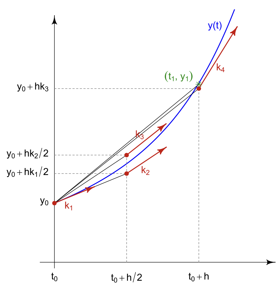
Even more elaborate, with 4 estimates per step, 1 for the value of \(f\) at its beginning, 2 for the middle, and 1 for the end. between \(t_i\) and \(t_{i+1}\) : \(y_{i+1}=y_i+\left(\frac{K_1}{6}+\frac{K_2}{3}+\frac{K_3}{3}+\frac{K_4}{6}\right)\), where
- \(K_1=h f\left(t_i, y_i\right)\)
- \(K_2=h f\left(t_i+\frac{h}{2}, y_i+\frac{K_1}{2}\right)\)
- \(K_3=h f\left(t_i+\frac{h}{2}, y_i+\frac{K_2}{2}\right)\)
- \(K_4=h f\left(t_i+h, y_i+K_3\right)\)
For our example case, - First step:
\[ \begin{aligned} & K_1=h\left(t_0-y_0\right)=-\frac{2}{3}, K_2=h\left(\left(t_0+\frac{h}{2}\right)-\left(y_0+\frac{K_1}{2}\right)\right)= \\ & -\frac{2}{9}, K_3=h\left(\left(t_0+\frac{h}{2}\right)-\left(y_0+\frac{K_2}{2}\right)\right)=-\frac{10}{27}, K_4= \\ & h\left(\left(t_1-\left(y_0+K_3\right)\right)=\frac{2}{81}, y_1=y_0+\left(\frac{K_1}{6}+\frac{K_2}{3}+\frac{K_3}{3}+\frac{K_4}{6}\right)=\frac{169}{243}\right. \end{aligned} \]
- Second step: \(K_1=-\frac{14}{729}, K_2=\frac{458}{2187}, K_3=\frac{874}{6561}, K_4=\)
\[ \frac{6622}{19683}, y_2=\frac{101866}{118098} \approx 0.8626 \]
- Third step: \(K_1 \approx 0.3139, K_2 \approx 0.4315, K_3 \approx 0.3923, K_4 \approx\) \(0.4968, y_3 \approx 1.2722\), which is the obtained estimate for \(y(t=2)\).
RK4 method sketch
Accuracy of these numerical methods
- For each method, the error in each step can be thought of as truncation of a Taylor series (as we saw explicitly for the Euler method), with a remainder term that has a derivative of \(f\) times a power of \(h\)
- The error in \(y_N=y(b)\) for each method is typically proportional to a positive power of \(h\) (less error if more steps are taken so that \(h\) is smaller). This power is the order of accuracy of the method (which is not the same as the order of the differential equation, explained above)
- Euler’s method has first-order accuracy
- Heun’s method has second-order accuracy
- The RK4 method has fourth-order accuracy (hence its name)
Implicit vs. Explicit ODE Methods
- Explicit methods:
Compute the next value directly from known quantities. Example (Euler’s Method):
\[ y_{n+1}=y_n+h \cdot f\left(t_n, y_n\right) \]
Simple, fast Can be unstable for stiff equations - Implicit methods:
Involve the unknown future value in the equation. Example (Backward Euler):
\[ y_{n+1}=y_n+h \cdot f\left(t_{n+1}, y_{n+1}\right) \]
More stable (good for stiff problems) Requires solving an equation at each step
Key difference: - Explicit: \(y_{n+1}\) computed directly - Implicit: \(y_{n+1}\) appears on both sides - may need iteration or root-finding
Implicit methods
- The methods so far for solving ODE IVPs were explicit, in that at each step, a formula for \(y_{i+1}\) is given in terms of quantities from the previous step
- By contrast, implicit methods have at each step a general formula for \(y_{i+1}\) that is not given in terms of only known values. This makes them more complicated to apply, but for some problems they can be accurate at larger step sizes, compared to explicit methods.
- The implicit methods we will discuss are
- The implicit Euler method, which has first-order accuracy
- The Crank-Nicolson method, which has second-order accuracy
Implicit Euler method
- Each step is \(y_{i+1}=y_i+h f\left(t_{i+1}, y_{i+1}\right)\)
- Note that \(y_{i+1}\) is unknown and appears on both sides of the equation, which is what makes this method implicit
- At least where \(f\) is a simple enough function, we can nevertheless find \(y_{i+1}\) at each step
- For our example, where \(f(t, y)=t-y\), each step is \(y_{i+1}=y_i+h\left(t_{i+1}-y_{i+1}\right)\), which we can write as \(y_{i+1}=\frac{y_i+h t_{i+1}}{1+h}\). So
- \(y_1=\frac{13}{15}\)
- \(y_2=\frac{79}{75}\)
- \(y_3=1.432\), which is the obtained estimate for \(y(t=2)\).
- Note that where the usual (explicit) Euler method gives an overestimate of the solution, the implicit method will usually give an underestimate, and vice versa.
Crank-Nicolson method
- Each step is \(y_{i+1}=y_i+\frac{h}{2}\left(f\left(t_i, y_i\right)+f\left(t_{i+1}, y_{i+1}\right)\right)-\) can be thought of as averaging the explicit and implicit Euler methods
- Note that \(y_{i+1}\) is unknown and appears on both sides of the equation, which is what makes this method implicit
- At least where \(f\) is a simple enough function, we can nevertheless find \(y_{i+1}\) at each step
- For our example, where \(f(t, y)=t-y\), each step is \(y_{i+1}=y_i+\frac{h}{2}\left(t_i+t_{i+1}-y_i-y_{i+1}\right)\), which we can write as \(y_{i+1}=\frac{\left(1-\frac{h}{2}\right) y_i+\frac{h}{2}\left(t_i+t_{i+1}\right)}{1+\frac{h}{2}}\). So
- \(y_1=\frac{2}{3}\)
- \(y_2=\frac{5}{6}\)
- \(y_3=1.25\), which is the obtained estimate for \(y(t=2)\).
- Tends to give results in between (and more accurate than either) the two Euler methods
Stability
- In some cases, explicit methods require a very small step size, otherwise the computed solution goes to infinity after many steps (numerical instability), while implicit methods can give a moderately accurate solution with a larger step size.
- The classic example of this is the ODE \(y^{\prime}(t)=-k y\), where \(k\) is some given positive number, and initial value \(y(0)=1\)
- The analytic solution is \(y(t)=e^{-k t}\) (exponential decay)
- Applying the Euler method to this problem gives \(y_{i+1}=y_i+h\left(-k y_i\right)=(1-h k) y_i\). So after \(n\) steps, the computed solution is \(y_n=(1-h k)^n\). This is a good approximation if \(h\) is small enough. But if \(h>\frac{2}{k}\), then \(|1-h k|>1\), so \(\lim _{i \rightarrow \infty}\left|y_i\right|=\infty\)
- By contrast, the implicit Euler method computed solution correctly goes to zero no matter how large \(h\) is: \(y_{i+1}=y_i+h\left(-k y_{i+1}\right)\), so \(y_{i+1}=\frac{y_i}{1+h k}\), and \(y_n=\frac{1}{(1+h k)^n}\)
Systems of first-order ODEs
Overview
- So far we saw how to use numerical methods for solving single first-order ODEs.
- However, engineering problems often involve systems of ODEs, as we saw, e.g., with the shear building model
- The same methods can be used to solve such systems also.
- Standard form for first-order ODE IVP systems is \(\left\{\begin{array}{l}z_1^{\prime}(t)=f_1\left(t, z_1(t), z_2(t) \cdots z_n(t)\right) ; z_1\left(t=t_0\right)=z_{1,0} \\ z_2^{\prime}(t)=f_2\left(t, z_1(t), z_2(t) \cdots z_n(t)\right) ; z_2\left(t=t_0\right)=z_{2,0} \\ \cdots \\ z_n^{\prime}(t)=f_n\left(t, z_1(t), z_2(t) \cdots z_n(t)\right) ; z_n\left(t=t_0\right)=z_{n, 0}\end{array}\right.\)
- Each unknown function \(z_i(t)\) has its own first-order differential equation (involving a known function \(f_i\) ) and inîtial value
- All initial values are at a common \(t_0\)
- The problem might be to find the values of some or all of the unknown functions at \(t=b\)
- More compactly, we can also write such systems in standard form using vector notation, as
\[ \mathbf{z}^{\prime}(t)=\mathbf{f}(t, \mathbf{z}) ; \mathbf{z}\left(t=t_0\right)=\mathbf{z}_0 \]
Example with Euler method
- Suppose we have \(\left\{\begin{array}{l}z_1^{\prime}(t)=t-z_2 \rightarrow z_1(0)=3 \\ z_2^{\prime}(t)=z_1 \rightarrow z_2(0)=2\end{array}\right.\)
- In vector form, \(\mathbf{f}=\binom{t-z_2}{z_1}, t_0=0, \mathbf{z}_0=\binom{3}{2}\)
- To find \(\mathbf{z}(2)\) with 3 equal-length steps ( \(h=\frac{2}{3}\) ), we would do
- First step: \(\mathbf{z}_1=\mathbf{z}_0+h\binom{t_0-z_{2,0}}{z_{1,0}}=\binom{\frac{5}{3}}{4}\)
- Second step: \(\mathbf{z}_2=\mathbf{z}_1+h\binom{t_1-z_{2,1}}{z_{1,1}}=\binom{-\frac{5}{9}}{\frac{46}{9}}\)
- Third step: \(\mathbf{z}_3=\mathbf{z}_2+h\binom{t_2-z_{2,2}}{z_{1,2}}=\binom{-\frac{83}{27}}{\frac{128}{27}}\), which is the obtained estimate for \(\mathbf{z}=\binom{z_1}{z_2}\) at \(t=2\).
Converting higher-order ODEs to first order
- Engineering problems can also involve higher derivatives, e.g., with the shear building model and with differential equations for beam deflection
- To use the above methods to solve a system with one or more higher-order ODEs, each ODE of order \(n>1\) needs to be converted into an equivalent system of \(n\) first-order ODEs.
Converting to first order: procedure
Start with the higher-order ODE in standard form:
\[ \frac{d^n y}{d t^n}=f\left(t, y, \frac{d y}{d t}, \frac{d^2 y}{d t^2}, \ldots, \frac{d^{n-1} y}{d t^{n-1}}\right) \]
with initial conditions
\[ y\left(t_0\right)=y_0^{(0)}, \frac{d y}{d t}\left(t_0\right)=y_0^{(1)}, \frac{d^2 y}{d t^2}\left(t_0\right)=y_0^{(2)}, \ldots, \frac{d^{n-1} y}{d t^{n-1}}\left(t_0\right)=y_0^{(n-1)} \]
Define a vector of unknown functions
\[ \mathbf{z}=\left(z_1, z_2, z_3, \ldots, z_n\right) \equiv\left(y, \frac{d y}{d t}, \frac{d^2 y}{d t^2}, \ldots, \frac{d^{n-1} y}{d t^{n-1}}\right) \]
- Write the system of first-order ODEs in terms of these unknowns as
\[ \begin{aligned} & z_1^{\prime}=z_2 \\ & z_2^{\prime}=z_3, \ldots \\ & z_{n-1}^{\prime}=z_n \\ & z_n^{\prime}=f\left(t, z_1, z_2, z_3, \ldots, z_n\right) \end{aligned} \]
- Write the initial conditions as \(z_i\left(t_0\right)=y_0^{(i-1)}, i=1,2, \ldots, n\)
Converting to first order: example
- Pendulum motion (with friction and a driving force) second-order ODE:
- \(\frac{d^2 \theta}{d t^2}+c \frac{d \theta}{d t}+\frac{g}{L} \sin (\theta)=a \sin (\Omega t)\)
- In standard form: \(\frac{d^2 \theta}{d t^2}=a \sin (\Omega t)-c \frac{d \theta}{d t}-\frac{g}{L} \sin (\theta)\)
- New unknown functions: \(z_1=\theta, z_2=\theta^{\prime}\)
- New system of first-order ODEs:
\[ \left\{\begin{array}{l} z_1^{\prime}(t)=z_2 \\ z_2^{\prime}(t)=a \sin (\Omega t)-\frac{g}{L} \sin \left(z_1\right)-c z_2 \end{array}\right. \]
- If the initial values are given as, e.g., \(\theta\left(t_0\right)=0, \theta^{\prime}\left(t_0\right)=0.1\), we would convert them to \(\left\{\begin{array}{l}z_1\left(t_0\right)=0 \\ z_2\left(t_0\right)=0.1\end{array}\right.\)