Motivation for Katz Centrality:
The problem with Eigen-centrality in directed networks
The Spectral Theorem: Why Symmetry Is a Gift in Network Analysis
- The spectral theorem says any real symmetric matrix has all real eigenvalues and a full set of orthogonal eigenvectors, so it can be written as \(A = Q\Lambda Q^{T}\): a clean rotation into a coordinate system where the matrix is just a diagonal stretch.
- Why networks care: undirected graphs have symmetric adjacency and Laplacian matrices, so the theorem applies and the eigenvectors become a natural basis (a “graph Fourier transform”) for any signal living on the nodes.
- It is the bedrock under a huge amount of method. Eigenvector centrality is well-posed (a unique, real, positive leading eigenvector), spectral clustering and graph partitioning split the graph along the low-eigenvalue eigenvectors, and diffusion, heat kernels, and random walks all decompose cleanly into independent eigen-modes.
- The intuition: orthogonal eigenvectors are non-interfering directions. A process on the graph can be broken into independent modes that each just decay or grow at their own rate, which is what makes the analysis tractable.
- The catch, and the thread through this unit: direction breaks symmetry. An asymmetric adjacency matrix can have complex eigenvalues, may not diagonalize, and splits left from right eigenvectors. Losing the spectral theorem is precisely why directed eigenvector centrality misbehaves and why fixes like Katz and PageRank exist.
Recall: Directed Acyclic Graph (DAG):
Recall: A cycle is a path that follows edge directions and returns to its starting node without repeating any edge or intermediate node along the way
A Directed Acyclic Graph (DAG) is a network made up of nodes (points or objects) and edges (arrows showing direction from one node to another), where:
- Directed means each edge has a one-way direction (like from A to B).
- Acyclic means you can never follow arrows and end up back where you started, there are no loops or cycles.
- In short: Information or influence flows forward, never circling back.
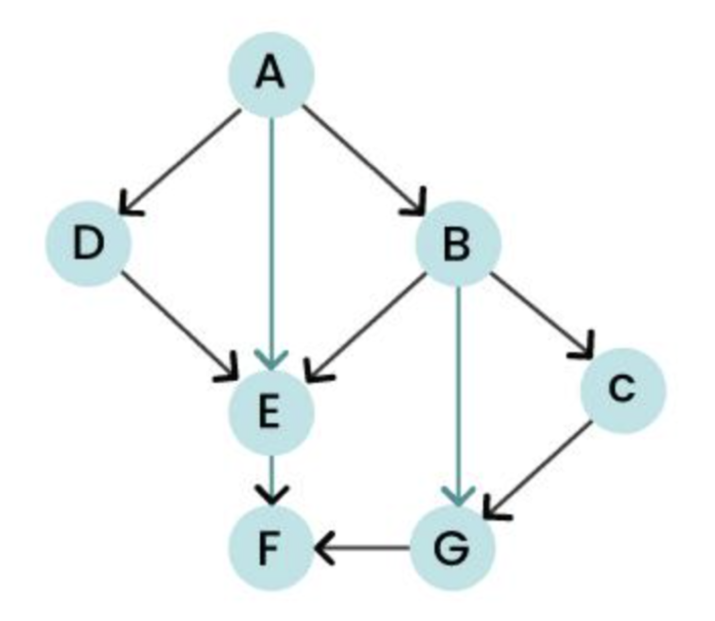
A Directed Acyclic Graph (DAG) contains a strict hierarchical flow with zero loops or cycles. Because influence can only move forward and never recirculate, traditional feedback-based centralities fail.
Jargon alert: Nilpotent Matrix
- Take the simplest acyclic chain: \(A \to B \to C\). Order the nodes as \([A, B, C]\).
\[ M = \begin{pmatrix} 0 & 1 & 0 \\ 0 & 0 & 1 \\ 0 & 0 & 0 \end{pmatrix} \]
- It is strictly upper triangular, so its eigenvalues are just the diagonal: \(0, 0, 0\).
- Multiply it by itself and the nonzero band marches off the edge: \(M^2\) has a single \(1\) in the corner, and \(M^3 = 0\).
- A matrix that powers down to zero is nilpotent. There is no positive leading eigenvalue for centrality to attach to.
Closer look: Why this matters
In Eigencentrality Importance Has to Circulate
- Eigenvector centrality is self-referential: you are important if important nodes point to you.
- For a node to hold a nonzero score, importance must flow in, get passed along, and eventually feed back.
- That feedback requires cycles. Cycles are the only thing that lets the recursion bootstrap a positive value from nothing.
- No cycles, no circulation, no score.
The Extreme Case: A Pure DAG
- A directed acyclic graph has no cycles anywhere, so importance can never loop back.
- Its adjacency matrix becomes nilpotent: reorder the nodes topologically and the matrix is strictly triangular.
- Every eigenvalue is zero, so the leading eigenvalue collapses to zero and the centrality is degenerate.
- This is the clean global failure
DAGs lacks cycles, a DAG’s adjacency matrix is nilpotent, meaning all of its eigenvalues are exactly zero (\(\lambda = 0\)), Which breaks Eigen-centrality formalism
Local “DAG-like” behavior
Recall: An SCC (strongly connected component) is a maximal set of nodes in a directed graph where every node can reach every other node by following edge directions.
It Is Not Only Pure DAGs that suffer
- Real directed graphs are full of cycles, yet the same breakdown still happens in pieces.
- The trick is to look at the strongly connected component (SCC) structure, not the whole graph at once.
- Local acyclicity inside a globally cyclic graph is enough to “starve a region”.
The SCC Picture
Collapse each SCC to a single node and you get the condensation, which is always a DAG.
Each nontrivial SCC has its own internal leading eigenvalue (its Perron root).
The global leading eigenvalue is just the largest of these, and the SCC that achieves it is dominant.
Centrality concentrates in the dominant SCC, flows downstream to whatever it can reach, and dies everywhere else.
Katz Centrality to the rescue
The solution to this problem is tweaking the formalism a bit to introduce a new centrality called Katz Centrality Leo Katz, 1953)
Introduction
Katz centrality extends degree centrality by considering not only a node’s immediate neighbors, but also neighbors-of-neighbors and more distant nodes. Influence propagates through the network along all possible walks, with longer walks receiving exponentially smaller weights.
- A node is important if it is reachable from many other nodes, with longer walks counting less than shorter ones
- Each node also receives a small amount of centrality “for free,” regardless of its connections
- Widely used in:
- Social network analysis (status, influence)
- Directed networks (citations, the web, gene regulation)
- Link prediction and recommendation systems
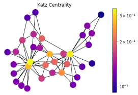
Adding a baseline
Katz centrality fixes this by adding a constant bias term (\(\beta\)), and an attenuation factor \(\alpha\) (weight given to neighbors’ scores) which grants every node a baseline injection of intrinsic importance.
\[x_i = \alpha \sum_{j} A_{ji} x_j + \beta\]
How it fixes the DAG: Source nodes (in-degree = 0) no longer get a score of zero; they retain a baseline score of \(\beta\).
The Mechanism: This baseline importance propagates down the DAG’s edges. A node’s score becomes a weighted sum of all upstream paths leading into it.
The Result: Katz centrality successfully ranks nodes in a DAG, establishing a clear hierarchy based on a node’s downstream position relative to its upstream ancestors.
Fixes the “Zero-In-Degree” Problem: In directed networks, standard eigenvector centrality assigns a score of 0 to any node with no incoming links, causing a domino effect that zeroes out downstream nodes.
Definition
The Katz centrality of node \(i\) is defined recursively:
\[ x_i = \alpha \sum_{j} A_{ji}\, x_j + \beta \rightarrow \mathbf{x} = \alpha A^T \mathbf{x} + \mathbf{\beta}\mathbf{1} \]
\(\mathbf{1}\) is the all-ones vector: a column vector with a \(1\) in every entry,
\(A\), adjacency matrix (\(A_{ji} = 1\) if there is an edge \(j \to i\))
\(\alpha\), attenuation factor (weight given to neighbors’ scores)
\(\beta\), constant baseline added to every node (typically \(\beta = 1\))
Analytic solution: (for \(\alpha < 1/\lambda_{max}\)): \(x=(I - \alpha A^{T})^{-1}\beta\mathbf{1}\)
Convergence Condition
The model converges only if
\[ \alpha < \frac{1}{\lambda_{\max}} \]
- where \(\lambda_{\max}\) is the largest eigenvalue of \(A\).
- If \(\alpha \geq 1/\lambda_{\max}\), the walk sums diverge and \((I - \alpha A^{T})\) is no longer invertible
- In practice: compute \(\lambda_{\max}\) first, then choose \(\alpha\) safely below \(1/\lambda_{\max}\) (e.g., \(\alpha = 0.85/\lambda_{\max}\))
- NetworkX defaults to \(\alpha = 0.1\), which is safe for many graphs but not all, always check!
Choosing the Baseline and the Attenuation Factor
- Baseline \(\beta\): almost always set to \(1\) uniformly, so every node starts with the same floor. Use a per-node dictionary only when you want a personalized or biased baseline.
- Attenuation \(\alpha\): the hard rule is \(\alpha < 1/\lambda_{max}\), where \(\lambda_{max}\) is the largest eigenvalue of the adjacency matrix. Cross this threshold and the path sum diverges and fails to converge.
- A common safe recipe is to compute \(\lambda_{max}\) and set \(\alpha\) to a fraction of \(1/\lambda_{max}\) (for example \(0.8\) to \(0.9\) of it), leaving headroom below the limit.
- NetworkX defaults:
alpha=0.1,beta=1.0. The small fixed \(\alpha\) is conservative and works for many graphs, but it can violate the convergence rule when \(\lambda_{max} > 10\), so check it on dense or high-degree networks. - Two limiting cases worth knowing: \(\beta = 0\) with \(\alpha = 1/\lambda_{max}\) recovers eigenvector centrality, and very small \(\alpha\) collapses Katz back toward plain in-degree.
Alternative form: Recursive and Walk-Sum Forms
- Recursive form. Each node’s score is a discounted echo of its in-neighbors’ scores, plus a baseline:
\[ x_i = \alpha \sum_{j} A_{ji}\, x_j + \beta \;\rightarrow\; \mathbf{x} = \alpha A^{T}\mathbf{x} + \beta\mathbf{1} \]
- Walk-sum form. Unrolling that recursion expands it into a contribution from directed walks of every length:
- Reading the sum. The \(k\)-th term counts every directed walk of length \(k\) ending at a node, each discounted by \(\alpha^{k}\), so longer paths matter less. The closed form on the right is what you get when that geometric series is summed.
\[ \mathbf{x} = \beta \sum_{k=0}^{\infty} \left( \alpha A^{T} \right)^{k} \mathbf{1} = \beta \left( I - \alpha A^{T} \right)^{-1} \mathbf{1} \]
- Substitute the recursion into itself. Replace \(\mathbf{x}\) on the right repeatedly; each pass peels off one baseline term and one extra factor of \(\alpha A^{T}\):
\[ \mathbf{x} = \beta\mathbf{1} + \alpha A^{T}\mathbf{x} = \beta\mathbf{1} + \alpha A^{T}\beta\mathbf{1} + (\alpha A^{T})^{2}\mathbf{x} = \beta\sum_{m=0}^{k}(\alpha A^{T})^{m}\mathbf{1} + (\alpha A^{T})^{k+1}\mathbf{x} \]
When \(\alpha < 1/\lambda_{max}\) the trailing term \((\alpha A^{T})^{k+1}\mathbf{x} \to 0\) as \(k \to \infty\), leaving exactly the walk-sum.
- Sum the geometric series. With spectral radius below \(1\), the matrix series collapses: \(\sum_{k=0}^{\infty}(\alpha A^{T})^{k} = (I - \alpha A^{T})^{-1}\), giving the closed form. (Equivalently, just rearrange the recursion: \((I - \alpha A^{T})\mathbf{x} = \beta\mathbf{1}\), so \(\mathbf{x} = (I - \alpha A^{T})^{-1}\beta\mathbf{1}\).)
Conceptual Picture
- Think of influence as something that flows along edges and decays with distance
- A walk of length \(k\) ending at node \(i\) contributes \(\alpha^k\) to node \(i\)’s score, where \(0 < \alpha < 1\) is an attenuation factor
- \(\alpha\) close to 0 → only immediate neighbors matter (behaves like degree centrality)
- \(\alpha\) close to its upper limit → long-range structure dominates (behaves like eigenvector centrality)
- The constant \(\beta\) gives every node a baseline score, so no node is ever “worth nothing”
- Interpretation: “You score a little just by existing, and more if important nodes point to you.”
Improvement over Eigenvector Centrality
Recall eigenvector centrality: \(\mathbf{x} = \frac{1}{\lambda_{\max}} A^{T} \mathbf{x}\), a node’s score is proportional to the sum of its neighbors’ scores.
Failure mode in directed graphs:
- A node with no incoming edges gets eigenvector centrality exactly zero
- Worse, that zero propagates: a node pointed to only by zero-score nodes also gets zero
- In a directed acyclic graph (DAG), every node ends up with score zero, the measure is useless
- Nodes outside strongly connected components are systematically zeroed out
Katz’s fix: the \(\beta\) term seeds every node with baseline centrality, which then flows along edges. Every node gets a meaningful, nonzero score.
When to Use Which?
| Situation | Recommended measure |
|---|---|
| Undirected, connected graph | Eigenvector, simple, parameter-free, well-behaved |
| Directed graph with strong connectivity (one big SCC) | Either works; eigenvector is simpler |
| Directed graph with sources, DAG structure, or many weak components | Katz, eigenvector collapses to zero |
| Citation networks, web graphs, follower networks | Katz (or PageRank) |
| You want a tunable “reach” parameter (local ↔︎ global) | Katz, adjust \(\alpha\) |
Rule of thumb: Eigenvector centrality is the special case; Katz is the safe general-purpose choice for directed networks.
Numerical Computation of Katz Centrality
Katz centrality calculates network influence via the matrix equation:
Is the Jacobi Method Used in Katz?
- Katz solves the linear system \((I - \alpha A^{T})\mathbf{x} = \beta\mathbf{1}\), and its usual iteration is:
\[ \mathbf{x}^{(k+1)} = \alpha A^{T}\mathbf{x}^{(k)} + \beta\mathbf{1} \]
- This is Jacobi in disguise. Jacobi divides each row by its diagonal, but here the diagonal of \(I - \alpha A^{T}\) is just \(1\), so that step does nothing and Jacobi collapses to plain “multiply and add.”
- Apply the Jacobi formula to this system properly and you get the Katz iteration back exactly: the diagonal is \(D = I\) and the off-diagonal part is \(-\alpha A^{T}\).
- The convergence conditions match too. Jacobi converges when the iteration matrix has spectral radius below \(1\), and here that matrix is \(\alpha A^{T}\), giving the familiar Katz bound \(\alpha < 1/\lambda_{max}\).
- Intuition: each sweep updates every node’s score from last sweep’s neighbor scores, then repeats until they settle. That is exactly one round of “spread importance, add the baseline.”
Closer look: How is Katz Centrality Computed?
\[\mathbf{x} = \alpha A^T \mathbf{x} + \mathbf{\beta}\]
Computing the centrality vector \(\mathbf{x}\) is fundamentally treated as solving a standard linear system, \(M\mathbf{x} = \mathbf{b}\), where \(M = (I - \alpha A^T)\) and \(\mathbf{b} = \mathbf{\beta}\). Computers use two primary approaches depending on graph size:
1. Direct Solver: LU Decomposition (Small/Medium Graphs)
The equation is algebraically rearranged to isolate \(\mathbf{x}\):
\[\mathbf{x} = (I - \alpha A^T)^{-1} \mathbf{\beta}\]
- Execution: Instead of calculating an expensive literal matrix inverse, the computer solves the linear system directly using LU Decomposition (e.g.,
scipy.linalg.solve). - Complexity: \(O(n^3)\) , highly exact, but too slow for massive networks.
2. Iterative Solver: Power Iteration / Jacobi (Large/Sparse Graphs)
To avoid heavy matrix operations on massive networks, the computer approximates the solution by iterating until convergence.
- Execution: 1. Initialize: \(\mathbf{x}^{(0)} = \mathbf{\beta}\)
- Update recursively: \(\mathbf{x}^{(k+1)} = \alpha A^T \mathbf{x}^{(k)} + \mathbf{\beta}\)
- Terminate when the update change drops below a threshold: \(\|\mathbf{x}^{(k+1)} - \mathbf{x}^{(k)}\| < \epsilon\)
- Complexity: \(O(m \cdot i)\) total, where \(m\) is the number of edges and \(i\) is the number of iterations. Driven by fast Sparse Matrix-Vector Multiplications (SpMV), making it highly memory-efficient.
A Toy Graph
A 4-node directed graph:
\[ 1 \to 2, \qquad 1 \to 3, \qquad 2 \to 3, \qquad 3 \to 4 \]
   (1) ──────► (2)
     \          │
      \         │
       ▼        ▼
       (3) ──► (4)
Adjacency matrix (row = source, column = target):
\[ A = \begin{pmatrix} 0 & 1 & 1 & 0 \\ 0 & 0 & 1 & 0 \\ 0 & 0 & 0 & 1 \\ 0 & 0 & 0 & 0 \end{pmatrix} \]
- This is a DAG: eigenvector centrality returns \(\mathbf{x} = \mathbf{0}\) for every node!
- Because \(A\) is nilpotent (\(\lambda_{\max} = 0\)), the Katz series converges for any \(\alpha\)
Worked Example: Hand Calculation
Set \(\alpha = 0.1\), \(\beta = 1\). Apply \(x_i = \beta + \alpha \sum_j A_{ji}\, x_j\) node by node (sum over in-neighbors). Since the graph is acyclic, we can solve sequentially:
Node 1 (no incoming edges):
\[ x_1 = 1 + 0.1 \cdot (0) = 1.000 \]
Node 2 (incoming from 1):
\[ x_2 = 1 + 0.1 \cdot x_1 = 1 + 0.1(1.000) = 1.100 \]
Node 3 (incoming from 1 and 2):
\[ x_3 = 1 + 0.1 \cdot (x_1 + x_2) = 1 + 0.1(1.000 + 1.100) = 1.210 \]
Node 4 (incoming from 3):
\[ x_4 = 1 + 0.1 \cdot x_3 = 1 + 0.1(1.210) = 1.121 \]
Result: \(\;x_1 = 1.000,\; x_2 = 1.100,\; x_3 = 1.210,\; x_4 = 1.121\)
Node 3 ranks highest, it receives walks from the most upstream structure. Eigenvector centrality would have ranked all four nodes equally at zero.
Verification in NetworkX
import networkx as nx

G = nx.DiGraph([(1, 2), (1, 3), (2, 3), (3, 4)])

katz = nx.katz_centrality_numpy(G, alpha=0.1, beta=1.0,
                                normalized=False)
print(katz)
Output:
{1: 1.0, 2: 1.1, 3: 1.21, 4: 1.121}- Note
normalized=False, by default NetworkX rescales the vector to unit Euclidean norm, which preserves the ranking but changes the raw values katz_centrality_numpysolves the linear system directly;katz_centralityuses power iteration (needsmax_iter/tol)
Limitations
- Choosing \(\alpha\) is arbitrary, results (and sometimes rankings) depend on it, and there is no universally principled value
- Convergence constraint: must verify \(\alpha < 1/\lambda_{\max}\), requiring an eigenvalue computation first
- Unbounded passing of influence: a high-Katz node passes its full score to every out-neighbor, a node with millions of out-edges (e.g., a directory page) inflates all its targets equally
- This motivates PageRank, which divides a node’s influence by its out-degree
- Cost: the matrix inverse \((I - \alpha A^{T})^{-1}\) is \(O(n^3)\); large graphs require iterative methods
- The \(\beta\) baseline means scores are not comparable across graphs of different sizes without normalization