Introduction to Network dynamics`
Recording
The following is a recording on this topic, I hope you find it useful!
Feel free to watch at 1.5x or 2x speed.
Note: If you find something missing or incorrect in the recording, then please let me know!
Introduction
Dynamic network fundamentals
Introduction
- What makes a network dynamic?
- Dynamic networks occur when any of the following change with time.
(1) network structure or sizee.g. node growth, death, new nodes joining/leaving the system, … etc(2) node attributes: e.g. individuals aging in a social network, amount of money in a bank account increasing or decreasing, etc- Often changes in node attributes are the result of something “flowing” through the network
- The system maybe subject to constraints in the form of conservation laws
(3) edge attributese.g. a “friendship score” describing an edge in a social network may get stronger or weaker with time.
- Dynamic Network data can arise from sampling
real world networksat different points in time OR by runningsimulationsof network phenomena
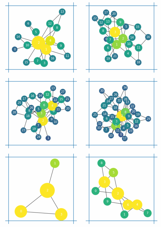
Example: Network growth
- Example of a dynamic
network structurevia network growth
- New nodes are added to the network as time progresses
Example: Thermal energy flow
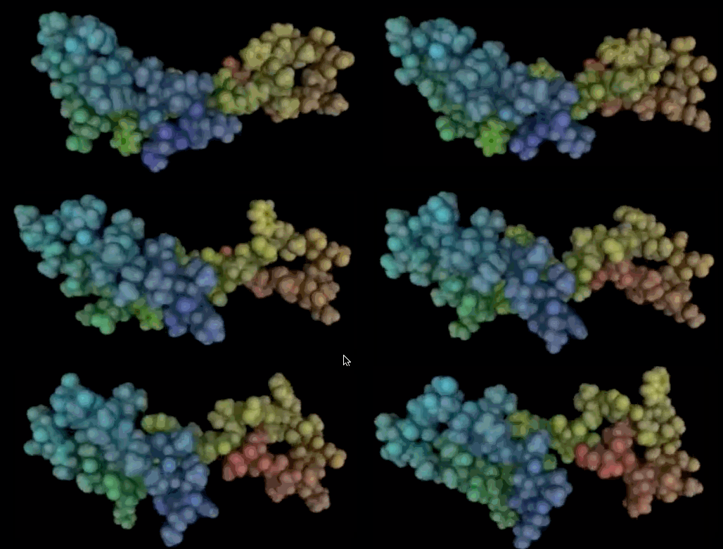
- Crystalline and amorphous solids are composed of networks of bonded atoms.
- As time progresses, positions, velocities, and energies (i.e nodal attributes) of the atoms change
- The theoretical formalisms of
Thermodynamicsandsolid-state physicsgovern the dynamics of such systems.
- The temporal evolution of such systems can be simulated using
Molecular dynamicsandmonte-Carlosimulation methodologies.
Temporal discretization
- A
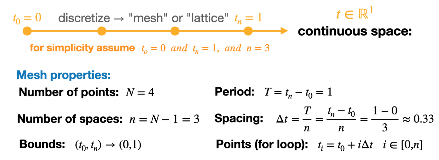
meshis a discretization of a geometric domain into small simple shapes, such as triangles, squares, or quadrilaterals. Meshes can be uniform or non-uniform. - Meshes are very important in applied math, since they from the domain on which our numerical functions are defined
- For the case of time, the time-domain mesh is just a single variable
Time-series data
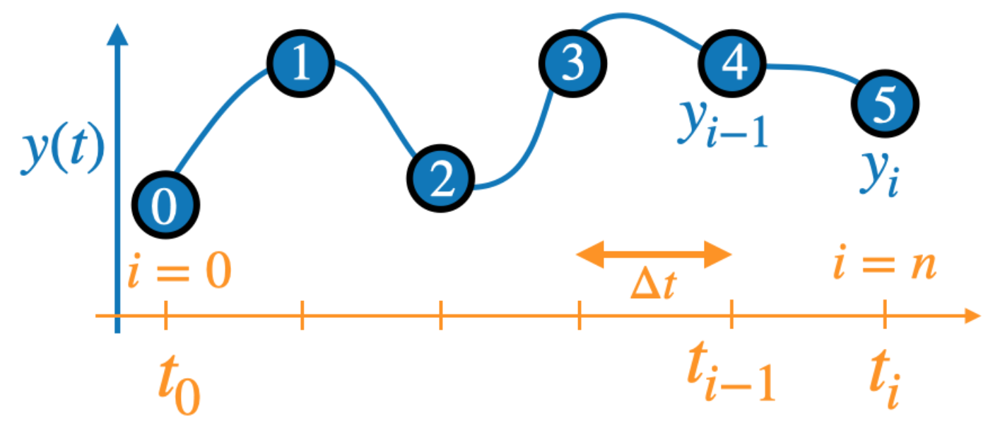
- Numeric time-series analysis requires us to define our time-series \(y(t)\) on a mesh.
- This is typically a uniform mesh, i.e. with a constant \(\Delta t\)
- (e.g. seconds, year, days, months, etc)
Storing temporal Network data
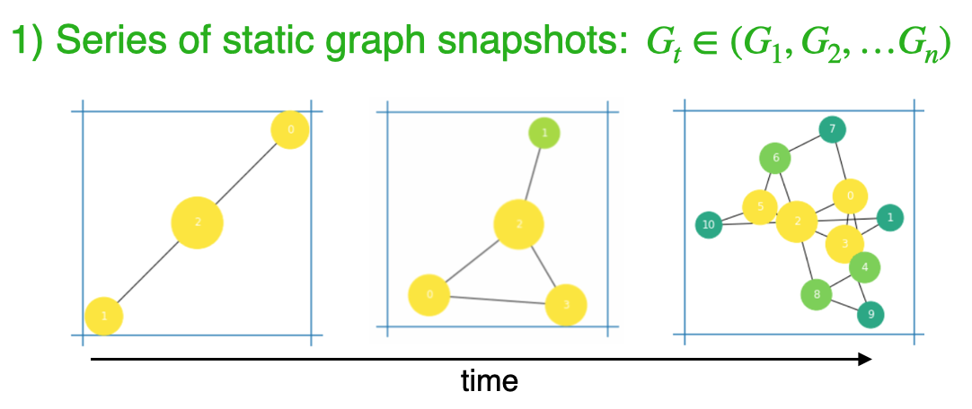
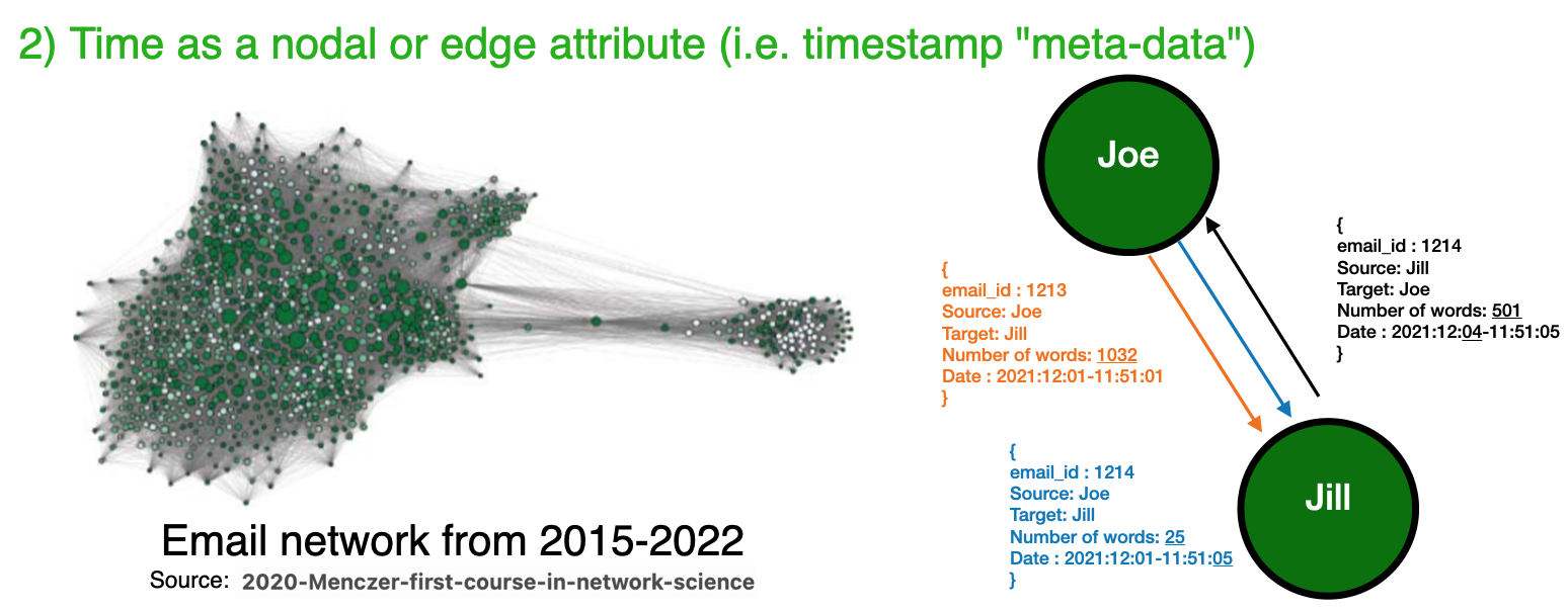
The following are common ways to store dynamic network data. Next week, we visualize dynamic networks in Gephi.
Communities are important in network dynamics
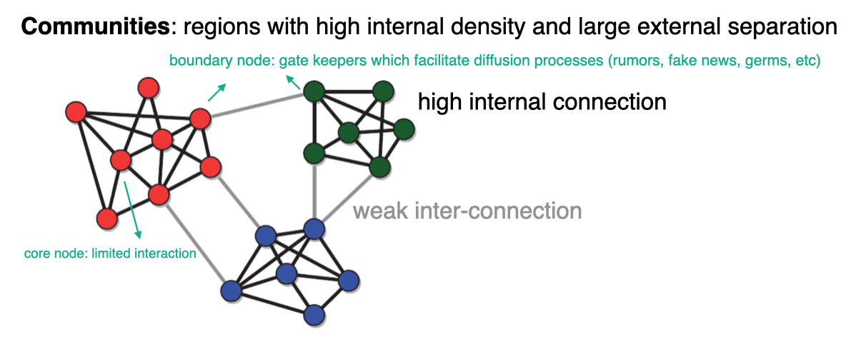
- Network structure plays an important role in the size and behavior of network diffusion processes
- This is because spread is facilitated within dense communities, but hindered by regions of low density (i.e. between) communities.
- Community boundaries act like walls to network spread
Dynamic network analysis methods
- Continuous: Let network continuously vary and evolve in time, visualize & analyst manually, draw determine trends and reach conclusions

- Time-windows: Divide network into static segments and analyze each individually (similar to what we’ve done in the past)

Dynamic network analysis methods
- Time-series approach: Treat network as a set of time-dependent attributes and apply time series analysis and visualization
- In this case, we can think of a dynamic network as a collection of inter-related time-series. One for each of the network properties which have a temporal dependence.
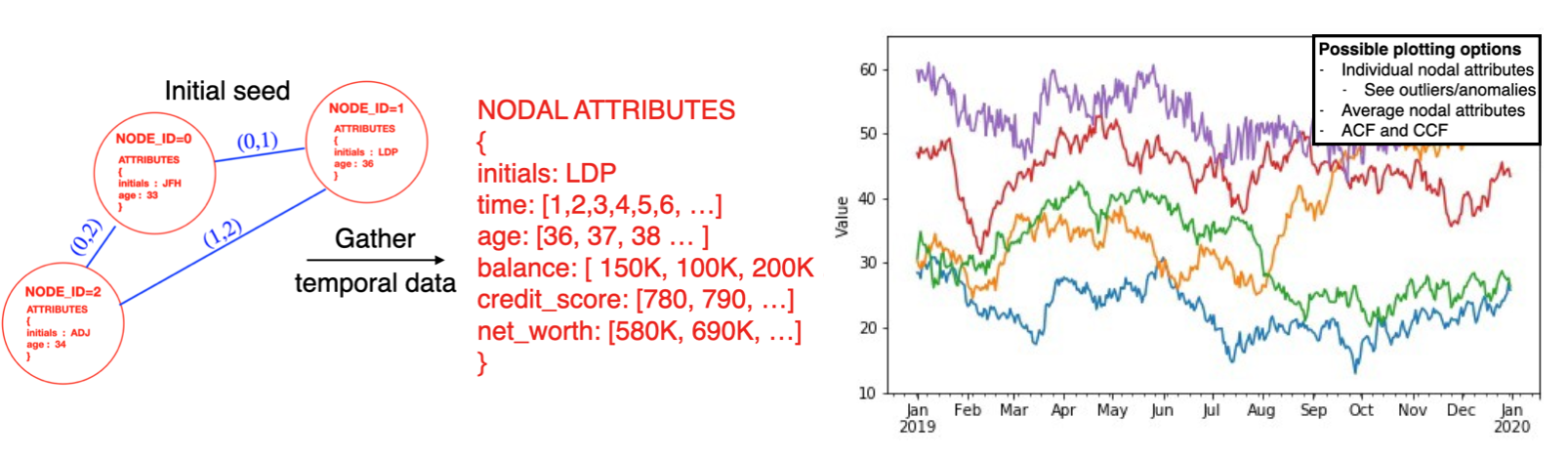
- From this prospective, we can use all of the standard visualization and modeling tools common to time-series analysis
Modeling dynamic systems
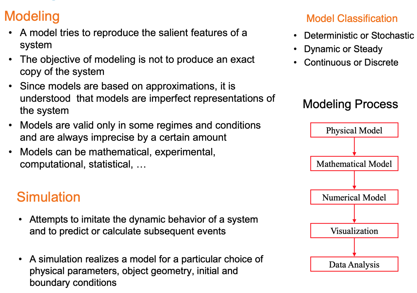
Simulations
Model categories
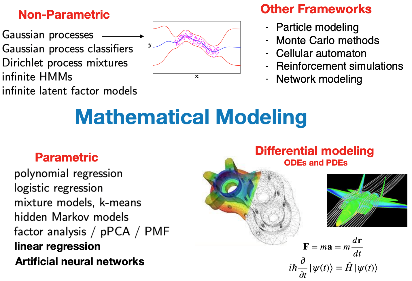
Modeling vs simulation
Example: Temporal differential model 1
- Often, dynamic processes are studied via
differential equations, where the independent variable is time.
- This is not the focus of today’s lecture, but it is an important branch of applied mathematics
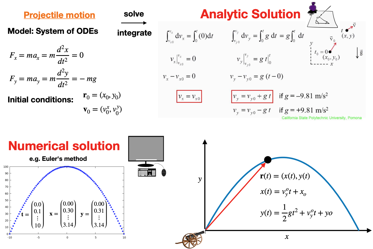
- On paper, differential equations treat time as continuous, but in the computer we must always discretize our variables.
Key components of dynamic simulations
- Initial conditions:
- Start with an initial network configuration (seed)
- Assume that a certain number of nodes (influencers) are initially activated.
- Time-steps: Discretize time and evolve the system forward one time-step at a time
- Rules of the game: Governing rules for the phenomena
- Inactive nodes can be activated (or not) according to some set of rules that depends on the presence of active neighbors and/or on other conditions and input parameters
- The outcome of this process is the creation of influence cascades, the activation in sequence of a subset of the nodes in the network.
- Cascades can range from a handful of nodes to global cascades involving a substantial proportion of the network.
- Validate your model
- Run simple cases of the model and compare, where possible, to real world data
- Exploration
- Run your simulation to explore new cases and phenomena
- Either on a laptop OR a supercomputer depending on the complexity of the simulation
- Post processing analysis
- Apply statistical analysis to the results and simulation outputs to make sense of them
Simulation update order
Important: The order in which nodes are updated should NOT affect the outcome of the model’s network dynamics.- There are multiple ways to implement the node update rules.
Fixed sequence: Same update sequence at each time-step (node-1,2 .. )- This is generally
badbecause it can introduce un-realistic artifacts
- This is generally
Asynchronous implementation: Nodes are evaluated in a different random sequence at each iteration.- Avoids biases that can result from always following the same sequence
Synchronous implementation:- The new activation state of each node for each iteration is determined using the activation values of the other nodes from the previous iteration; all of the nodes are updated at the end of the iteration. The order is irrelevant in this case.
Source: Menczer1
Boundary conditions
- Boundary conditions (BC) are another important “ingredient” in many simulation and differential models
- The BC encode specific instructions regarding how quantities should “interact” with the “edge” of the simulation cell.
- “Boundary conditions” are typically “fixed” or “periodic”
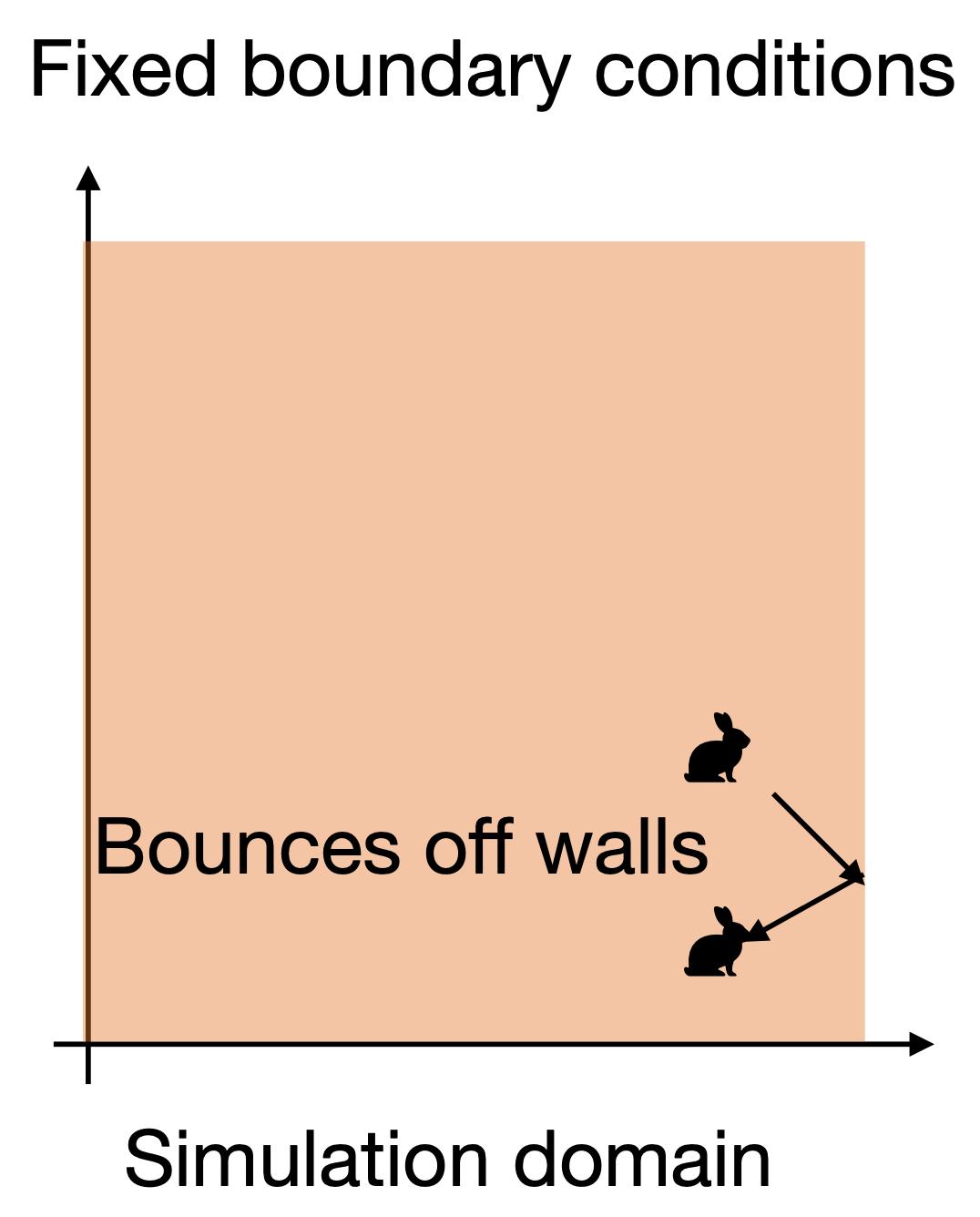
Fixed Boundaries
- Simulates a rigid edge: i.e. bounce off the edge or interact with fixed nodes
Periodic boundary conditions
- With periodic boundary conditions, if something leaves the simulation domain, it wraps back around and re-enters the other side (Out one side, in the other)
NOTE:Not all network simulations require boundary conditions (some do, some don’t)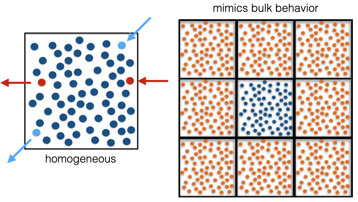
Interaction cutoffs
- To accelerate computation, it is also common in simulations to only consider a finite set of interactions
- For example, in a physical atomic simulation, you might only consider the closest atoms within some search radius
NOTE:Not all network simulations require interaction cut-offs (some do, some don’t)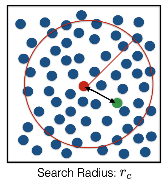
Network flux and diffusion mechanisms
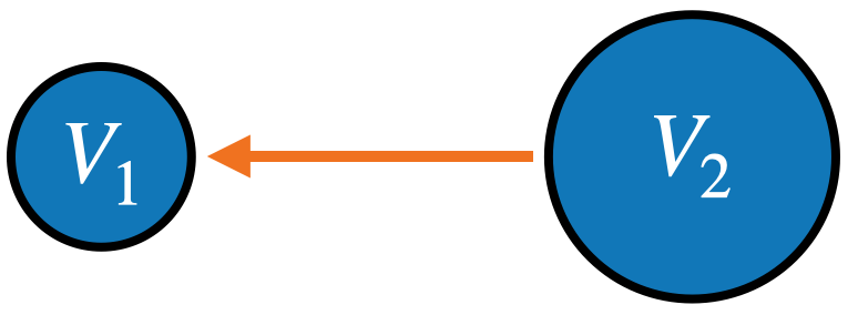
Definition: Flux is the action or process of flowing.
Overview
- Something flowing through the network is a common source of a dynamic process.
For example, Oil flowing between refineries, kinetic energy flowing between atoms (thermal conduction), people flowing between cities, etc
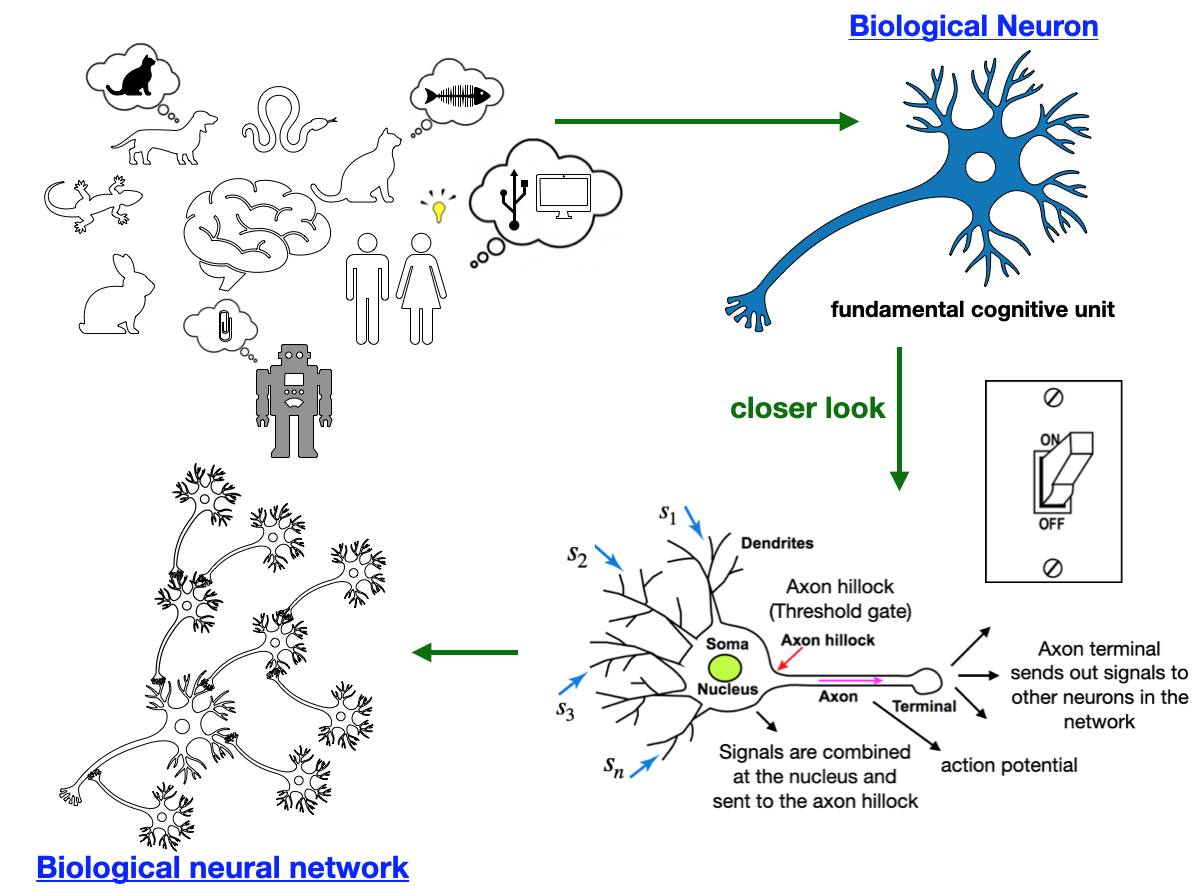
Example: Biological neural network
Neuronal firing causes communication between neurons via electrical impulses (current) and neurotransmitters (molecules).


Biological neural networks
Continuous flow
- Some quantities can flow (vary)
continuously(e.g water flowing through a pipe) - The flow is facilitated by a transportable medium (e.g mass, money, electrons, energy)
Example: Water flow 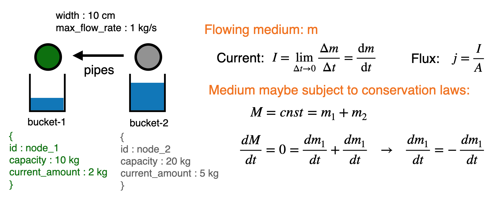
Discrete flow
- Some quantities are inherently
discreteand can NOT vary continuously.- These are generally
binaryormulti-classcategorical quantities: For example, illness, ideas/memes, opinions, etc
- These are generally
- As time progresses, part of they system transitions from one discrete state to another
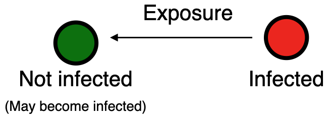
Example: Discrete (binary) transmission.
spreading of social effects is often called social contagion, because such processes often resemble disease transmission
Example: Physical diffusion
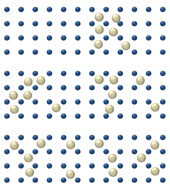
- Atomic diffusion is a diffusion process whereby the random, thermally-activated movement of atoms in a solid results in the transport of atoms
- If the occupation sites are treated as discrete locations, then this phenomenon can be modeled as a discrete process.
Diffusion mechanisms
- When something
flows, we generally want to understand why it is happening and describe the process mathematically. - One common mechanism is caused by an in-equality (gradient) in some quantity in different regions of the network.
- In some systems there is an
equilibriumstate. If the system is in anon-equilibriumstate, then there will be adriving forceto re-distribute resources and re-establish equilibrium.
Example: We are often exposed to ideas and/or germs via friends/neighbors. The extent of the difference between our ideas, and our neighbors, may trigger a diffusion event
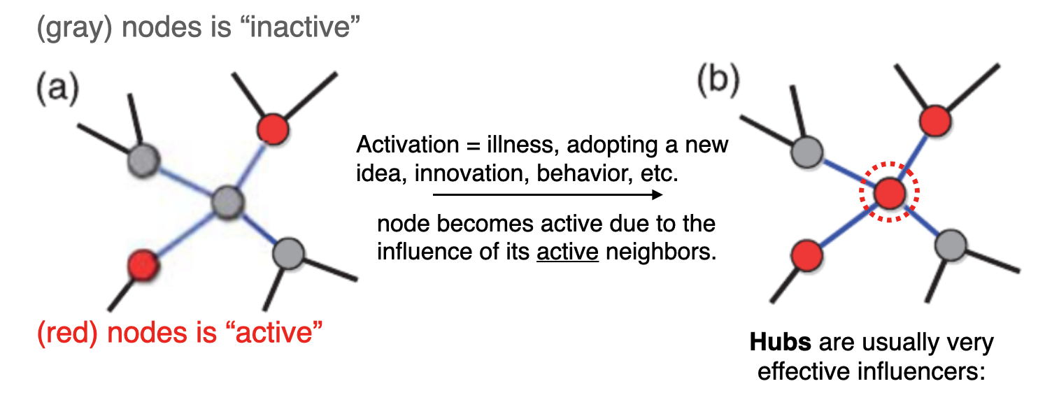
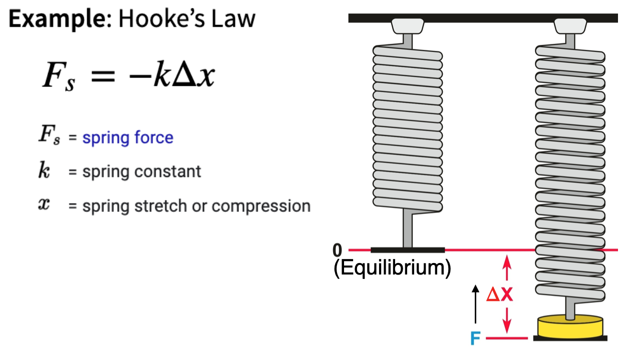
Linear restoring forces
- While not always the case, often it is reasonable to assume a linear dependence between variables.
- In fact, any function can be locally approximated as a linear function (i.e. the first order term in the
Taylor series) \[f(x)=f(a)+f^{\prime}(a)(x-a)+\frac{f^{\prime \prime}(a)}{2 !}(x-a)^2+\ldots\] - In physics, the restoring force of some quantity often depends linearly on a perturbation \(\Delta x\) in some other quantity
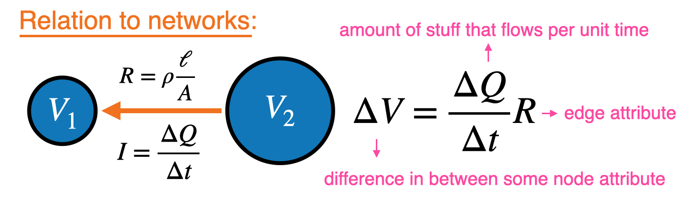
- The same is also often true of the flux in some quantity for restoring forces
- The linearity introduces a constant of proportionality \(k\)
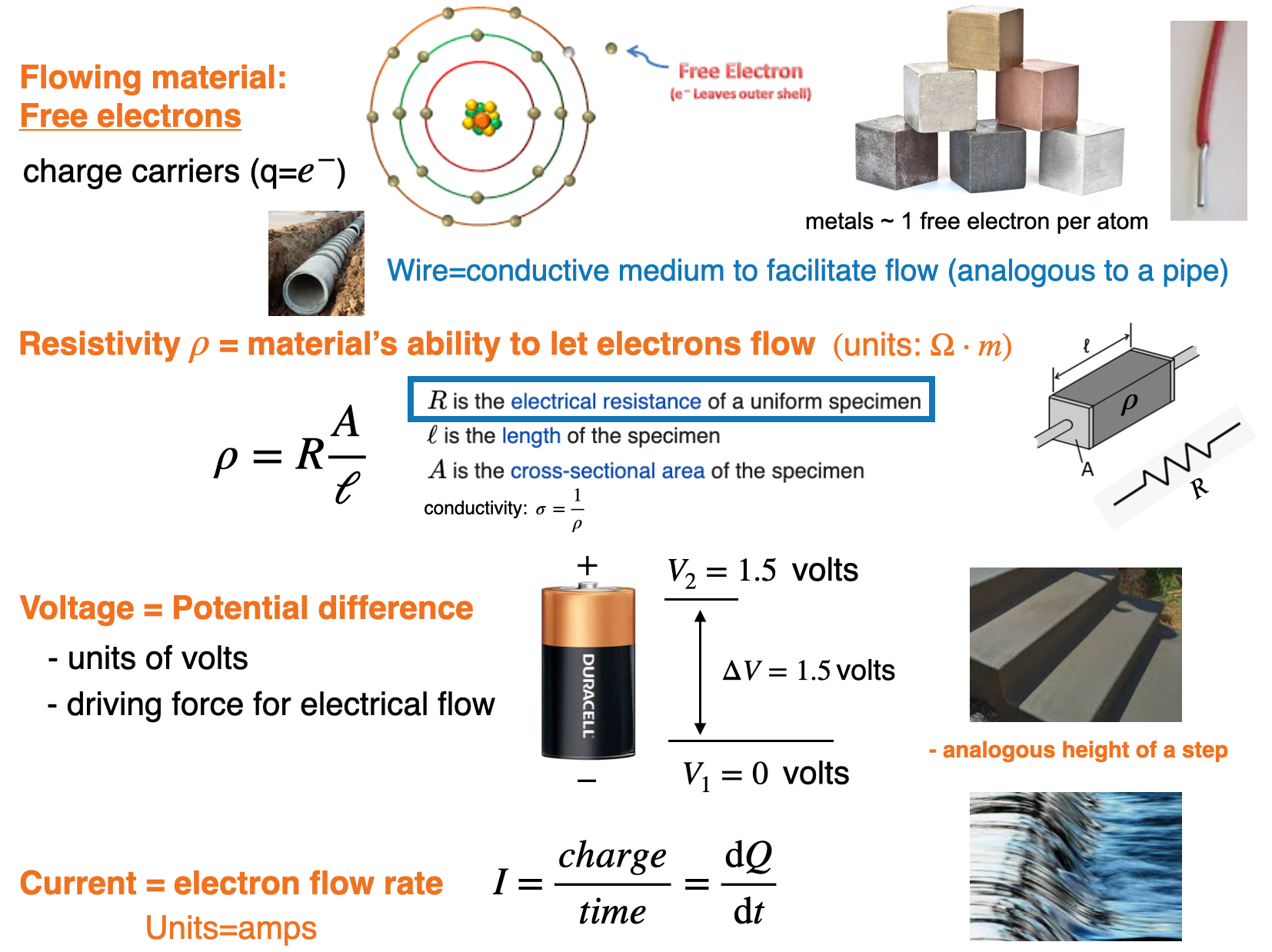
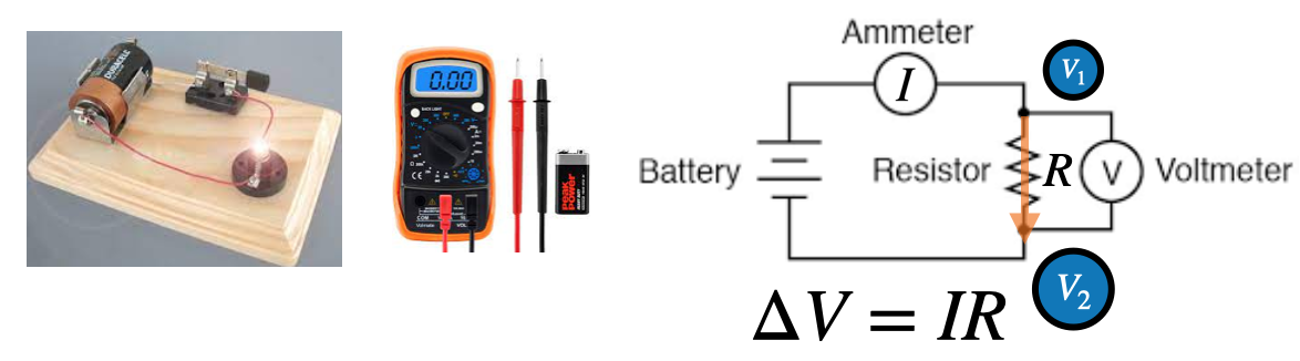
Example: Electrical flow
Simple electrical circuit
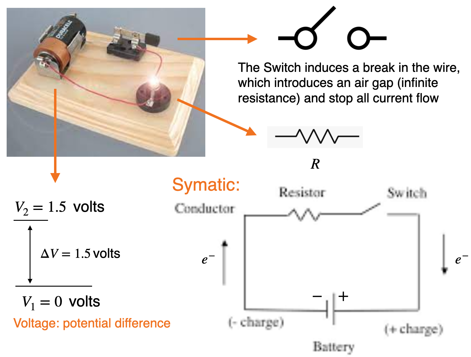
Ohms law
Ohm's law\(\rightarrow\) The current through a conductor, between two points, isdirectly proportionalto the voltage (potential difference) across the two points.
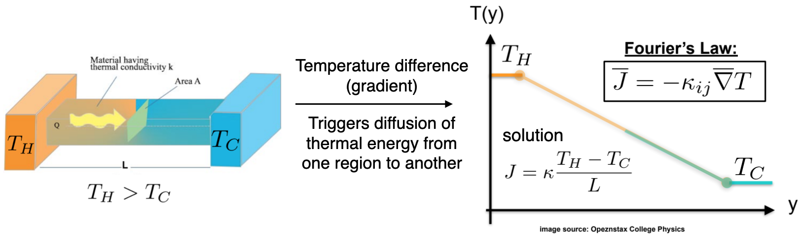
Thermal diffusion mechanism
Conductionis the process by which heat is transferred from the hotter end to the colder end of an object. The ability of the object to conduct heat is known as its thermal conductivity, and is denoted k.- The law of heat conduction, also known as Fourier’s law, states that the rate of heat transfer through a material is proportional to the negative gradient of temperature, with respect to space.