ANLY-645: Week-06

Chapter-6: Communities

Slide download

Click here to download the relevant notebook(s) for these slides

–>

Break

Lets take a 10 minute break before moving onto the lab.

Lab presentation

Student lab presentation

Lab Demonstration

Partitions, Modularity, Zachary’s Karate Club, Girvan-Newman clustering algorithm

Partitions

  • Recall: A partition of a graph is a separation of its nodes into disjoint groups.
  • There are two trivial partitions:
    1. The partition with one set containing every node;
    2. The partition with N sets, each containing a single node.
  • A valid partition thus contains between 1 and N sets.

Import & load network

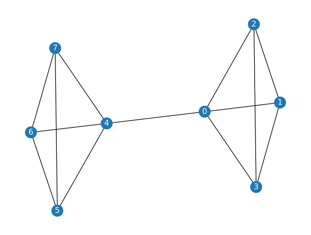
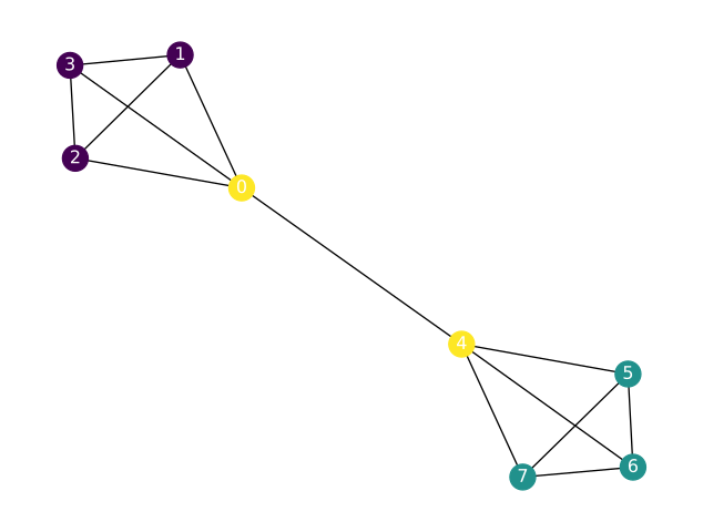
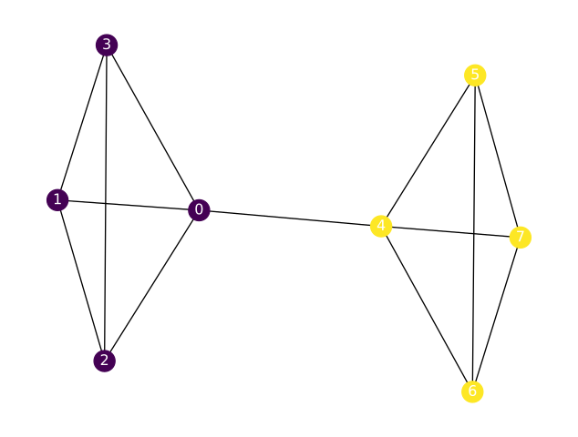
  • We will use a simple toy graph, with two fully connected communities, each with four nodes, connected by a single link
# IMPORT 
import random
import networkx as nx
import matplotlib.pyplot as plt
import numpy as np

# LOAD & DRAW
G=nx.read_adjlist('network.txt')
nx.draw(G, with_labels=True, font_color="white")

# CONVERT STRING LABELS TO INTS 
# print(G.nodes)
G=nx.convert_node_labels_to_integers(G, first_label=0); #print(G.nodes)

Example: Partition

  • Formally, a partition is a list of sets such that every node is in exactly one set, which is the case here.
  • The following is an example of a partition of the nodes in our network
  • Notice how the partitions are stored as a list of dictionaries containing node-IDs for the three partitions
partition = [
    {1, 2, 3},
    {5, 6, 7},
    {0, 4},
]

NetworkX can verify that our partition is valid:

print(partition)
print("\n",nx.community.is_partition(G, partition))
[{1, 2, 3}, {5, 6, 7}, {0, 4}]

 True

Aside: Python enumerate

  • In Python, a for loop is usually written as a loop over an iterable object. This means you don’t need a counting variable to access items in the iterable.
  • Sometimes, though, you do want to have a variable that changes on each loop iteration.
  • Rather than creating and incrementing a variable yourself, you can use Python’s enumerate() to get a counter and the value from the iterable at the same time!
# WITHOUT ENUMERATE 
idx=0;
for i in [0,10,20,30]:
    idx+=1
    print(idx,i)
1 0
2 10
3 20
4 30
# WITH ENUMERATE 
for idx,item in enumerate([0,10,20,30]):
    print(idx,item)
0 0
1 10
2 20
3 30

Partition maps

  • When developing community detection algorithms, we often use a partition map
    • i.e a dictionary mapping node names to a partition index.
  • This is useful for quickly comparing if two nodes are in the same cluster in the partition:
partition_map = {}

for idx, cluster_nodes in enumerate(partition):
    print(idx,cluster_nodes)
    for node in cluster_nodes:
        partition_map[node] = idx

partition_map
0 {1, 2, 3}
1 {5, 6, 7}
2 {0, 4}
{1: 0, 2: 0, 3: 0, 5: 1, 6: 1, 7: 1, 0: 2, 4: 2}

In this dictionary, the keys are the node names and two nodes will have the same value if they are in the same partition:

print(partition_map[1] == partition_map[2])
print(partition_map[0] == partition_map[7])
True
False

Aside: list comprehension

  • List comprehension provides a more concise syntax when creating a new list based on the values of an existing list,
# WITH LIST COMPREHENSION 
list1=[0,1,2,3,4,5]
list2=[]
for i in range(0,len(list1)):
    list2.append(2*list1[i])
print(list2)
[0, 2, 4, 6, 8, 10]
# WITH LIST COMPREHENSION-1
list3=[2*list1[i] for i in range(0,len(list1))]
print(list3)
[0, 2, 4, 6, 8, 10]
# WITH LIST COMPREHENSION-2
list4=[2*value for value in list1]
print(list4)
[0, 2, 4, 6, 8, 10]

Visualizing partitions

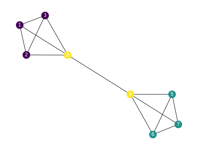
We can visualize partitions by coloring nodes with their partition membership:

node_colors = [partition_map[n] for n in G.nodes]
print(node_colors)
nx.draw(G, node_color=node_colors, with_labels=True, font_color="white")
[2, 0, 0, 0, 2, 1, 1, 1]

Utility function

  • We can make a function that takes a graph, and a given partition, and generates a color coded plot
def plot_partition(G,partition):
    #BUILD PARTITION-MAP
    partition_map = {}
    for idx, cluster_nodes in enumerate(partition):
        for node in cluster_nodes:
            partition_map[node] = idx
    #PLOT
    node_colors = [partition_map[n] for n in G.nodes]
    nx.draw(G, node_color=node_colors, with_labels=True, font_color="white")
    plt.show()

Explore partitions

Run the following code to test your plotting function

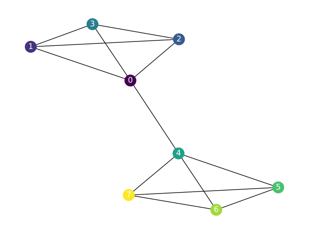
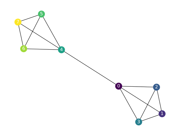
#PARTITION-1: (singletons)
partition = [{0},{1},{2},{3},{4},{5},{6},{7}]
plot_partition(G,partition)

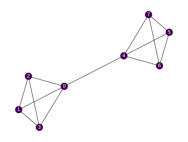
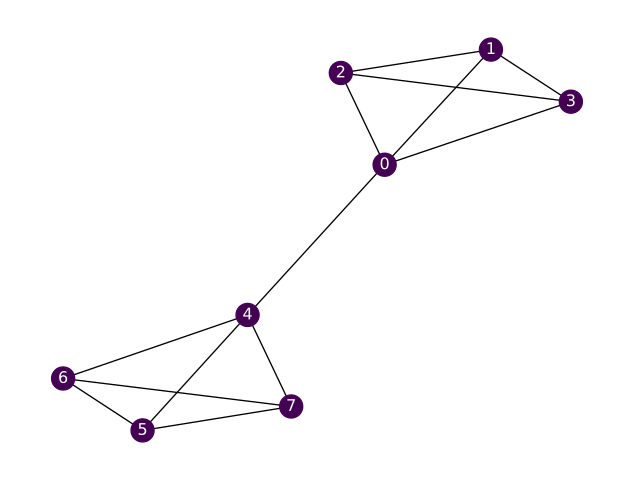
#PARTITION-2: (full network)
partition = [{0,1,2,3,4,5,6,7}]
plot_partition(G,partition)

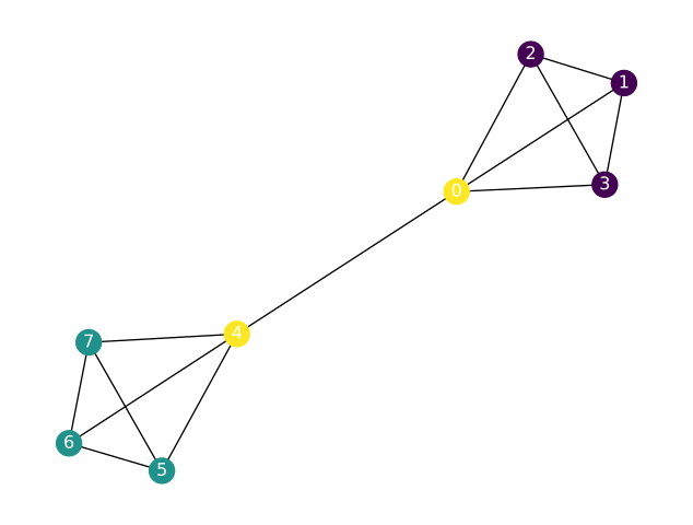
#PARTITION-3:
partition = [{1, 2, 3},{5, 6, 7},{0, 4}]
plot_partition(G,partition)

Modularity: Overview

  • At a high level, network community detection consists of finding a partition that achieves good separation between the groups of nodes.
  • Before we get into how to find good partitions of a graph, we need an objective – a way to measure how good the partition is.
  • Modularity is one such objective function.
  • The modularity of a graph partition compares the number of intra-group edges with a random baseline.
  • Higher modularity scores correspond to a higher proportion of intra-group edges
    • Higher modularity = better separation of groups
    • A random partition will have a modularity around zero
  • For weighted undirected networks, as described in the text, we have

\[ Q_w=\frac{1}{W}\sum_C \left(W_C-\frac{s_C^2}{4W}\right) \]

where

  • \(W\) is the total weight of the links of the network,
  • \(W_C\) the total weight of the internal links of cluster \(C\), and
  • \(s_C\) the total strength of the nodes of \(C\).

Explore modularity

  • NetworkX provides a modularity function, let’s compare several partitions
#PARTITION-1: (singletons)
str1=""
partition = [{0},{1},{2},{3},{4},{5},{6},{7}]
plot_partition(G,partition)
str1+=str(np.round(nx.community.quality.modularity(G, partition),3))+"      "

#PARTITION-2: (full network)
partition = [{0,1,2,3,4,5,6,7}]
plot_partition(G,partition)
str1+=str(np.round(nx.community.quality.modularity(G, partition),3))+"      "

#PARTITION-3:
partition = [{1, 2, 3},{5, 6, 7},{0, 4}]
plot_partition(G,partition)
str1+=str(np.round(nx.community.quality.modularity(G, partition),3))+"      "

# PARTITION-4
partition = [{0, 1, 2, 3},{4, 5, 6, 7}]
plot_partition(G,partition)
str1+=str(np.round(nx.community.quality.modularity(G, partition),3))+"      "

print("modularity values: \n", str1)

modularity values: 
 -0.127      0.0      0.204      0.423      

Zachary’s Karate Club

Overview

  • When writing and testing community-detection algorithms, it helps to make use of benchmark networks: graphs with a known, “natural” community structure.
  • Perhaps the most famous benchmark graph is Zachary’s Karate Club.
    • It contains 34 nodes, representing members of a karate club whose interactions were monitored over a period of three years by researchers.
    • Links in this graph connect individuals interacting outside club activities, a proxy for social ties.
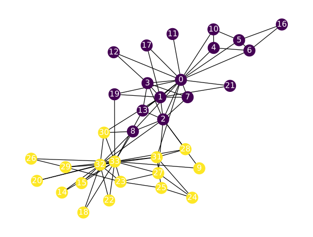
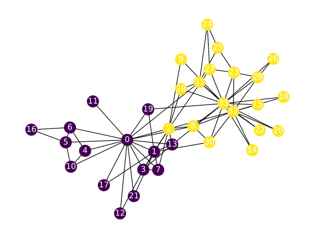
    • During the course of the study, a conflict between the instructor Mr. Hi (node 0) and the president, or Officer (node 33) led to a split of the club into separate groups led by Mr. Hi and Officer.
  • In this case we know whom each member of the group followed after the split, providing empirical community labels: those members who followed Mr. Hi are said to be one community and those following the Officer make up the other.
  • For this graph, we assume that the post-split group composition was largely driven by the social ties: members of the same friend groups would want to be part of the same club after the split.
  • We thus expect a good community-detection algorithm to predict the post-split group composition with high accuracy.
  • Zachary’s karate club is such a popular benchmark graph that it has its own function in NetworkX:

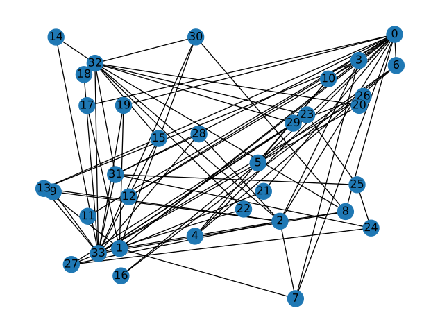
Load and draw network: Random

K = nx.karate_club_graph()

# RANDOM 
nx.draw(K, pos=nx.random_layout(K), with_labels=True)
plt.show()

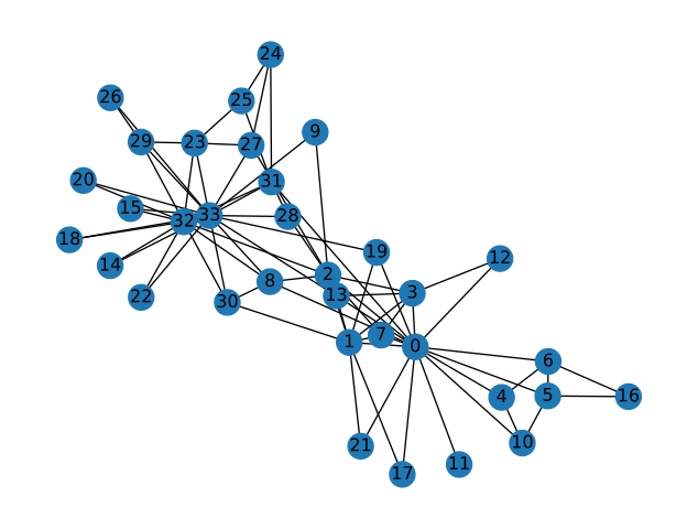
Load and draw network: Force directed

  • Recall: Instructor Mr. Hi is node-0 and the president, or Officer is node-33.

# FORCE DIRECTED (Fruchterman-Reingold force-directed algorithm.)
nx.draw(K, pos=nx.spring_layout(K, iterations=250, threshold=0.00001), with_labels=True)
plt.show()

Aside: Assigning node attributes

  • Each node in a NetworkX graph has a dictionary of attributes associated with it. (empty by default)
  • This dictionary can hold arbitrary data about a node.
  • We can get the attributes for a single node by giving the node name to the nodes object.
# CREATE GRAPH WITH ATTRIBUTES
G1=nx.Graph()
G1.add_node(0, D=-1)
G1.add_node(1, D=-2)
print(G1)

# ACCESS ATTRIBUTES 
print(G1.nodes[0]["D"])
print(G1.nodes[1]["D"])

# OVERWRITE ATTRIBUTE 
G1.nodes[0]["D"]=100
print(nx.get_node_attributes(G1, 'D'))
Graph with 2 nodes and 0 edges
-1
-2
{0: 100, 1: -2}

Explore node attributes

  • Each node in this graph has a 'club' attribute, indicating whether the member followed the instructor or the president after the split:
print(K.nodes)
for i in range(0,len(K.nodes)):
    print(K.nodes[i])
[0, 1, 2, 3, 4, 5, 6, 7, 8, 9, 10, 11, 12, 13, 14, 15, 16, 17, 18, 19, 20, 21, 22, 23, 24, 25, 26, 27, 28, 29, 30, 31, 32, 33]
{'club': 'Mr. Hi'}
{'club': 'Mr. Hi'}
{'club': 'Mr. Hi'}
{'club': 'Mr. Hi'}
{'club': 'Mr. Hi'}
{'club': 'Mr. Hi'}
{'club': 'Mr. Hi'}
{'club': 'Mr. Hi'}
{'club': 'Mr. Hi'}
{'club': 'Officer'}
{'club': 'Mr. Hi'}
{'club': 'Mr. Hi'}
{'club': 'Mr. Hi'}
{'club': 'Mr. Hi'}
{'club': 'Officer'}
{'club': 'Officer'}
{'club': 'Mr. Hi'}
{'club': 'Mr. Hi'}
{'club': 'Officer'}
{'club': 'Mr. Hi'}
{'club': 'Officer'}
{'club': 'Mr. Hi'}
{'club': 'Officer'}
{'club': 'Officer'}
{'club': 'Officer'}
{'club': 'Officer'}
{'club': 'Officer'}
{'club': 'Officer'}
{'club': 'Officer'}
{'club': 'Officer'}
{'club': 'Officer'}
{'club': 'Officer'}
{'club': 'Officer'}
{'club': 'Officer'}

Visualize “ground truth” partition

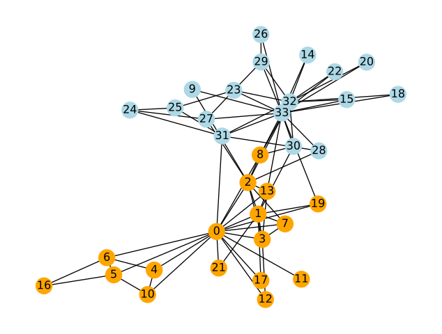
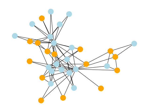
  • We can visualize these labels by coloring each node according to its 'club' attribute:
K = nx.karate_club_graph()
club_color = {
    'Mr. Hi': 'orange',
    'Officer': 'lightblue',
}
node_colors = [club_color[K.nodes[n]['club']] for n in K.nodes]
nx.draw(K, pos=nx.spring_layout(K),node_color=node_colors, with_labels=True)

  • The separation looks good (few inter-community links vs intra-community links)

Convert to a partition data-structure

  • Let’s create a graph partition based on these labels and measure its modularity.
  • We can do this by creating a dictionary of two sets, one for each value of the nodes’ 'club' attribute, then assigning the nodes to the corresponding set.
groups = {
    'Mr. Hi': set(),
    'Officer': set(),
}

for n in K.nodes:
    club = K.nodes[n]['club']
    groups[club].add(n)
    
print(groups)
{'Mr. Hi': {0, 1, 2, 3, 4, 5, 6, 7, 8, 10, 11, 12, 13, 16, 17, 19, 21}, 'Officer': {32, 33, 9, 14, 15, 18, 20, 22, 23, 24, 25, 26, 27, 28, 29, 30, 31}}

Using the dictionary’s .values() method, we get the list that defines our partition:

empirical_partition = list(groups.values())
print(empirical_partition)
[{0, 1, 2, 3, 4, 5, 6, 7, 8, 10, 11, 12, 13, 16, 17, 19, 21}, {32, 33, 9, 14, 15, 18, 20, 22, 23, 24, 25, 26, 27, 28, 29, 30, 31}]

Explore “ground truth” partition modularity

plot_partition(K,empirical_partition)
nx.community.is_partition(K, empirical_partition)

True

Since our partition is indeed a valid partition, we can get the modularity of this partition:

print(nx.community.quality.modularity(K, empirical_partition))
0.39143756676224206

This is a relatively high modularity, which is what we expect.

Random partition: Create list

  • For comparison, let’s generate a random partition of this network and check its modularity.
  • We would expect a modularity close to zero in this case.
  • First we generate a sample of 17 nodes, half the total number of nodes, and assign them to one community.
  • Our second community then includes the nodes in the graph not in the first community.
  • We can use some set arithmetic to do this concisely:
random_nodes = random.choices(list(K.nodes), k=17)
random_partition = [set(random_nodes),
                    set(K.nodes) - set(random_nodes)]
print(random_partition)
[{5, 6, 7, 8, 9, 10, 11, 12, 14, 17, 21, 23, 28, 29, 30}, {0, 1, 2, 3, 4, 13, 15, 16, 18, 19, 20, 22, 24, 25, 26, 27, 31, 32, 33}]

Random partition: Visualize and compute modularity

We can visualize this partition and observe that the communities are much less natural-looking, as we would expect from a random assignment.

random_node_colors = ['orange' if n in random_nodes else 'lightblue' for n in K.nodes]
nx.draw(K, pos=nx.spring_layout(K), node_color=random_node_colors)

And finally we can test the modularity of this partition:

print(nx.community.quality.modularity(K, random_partition))
-0.057232810479563676
  • Since this is a random process the modularity should be close to zero, as expected

Girvan-Newman clustering

Using NetworkX

Overview

  • The Girvan–Newman algorithm detects communities by progressively removing edges from the original graph.
  • The algorithm removes the “most valuable” edge, traditionally the edge with the highest betweenness centrality, at each step.
  • As the graph breaks down into pieces, the tightly knit community structure is exposed
  • The result can be depicted as a dendrogram.
  • Finds communities in a graph using the Girvan–Newman method.
  • girvan_newman(G, most_valuable_edge=None)
    • Input
      • Function that takes a graph as input and outputs an edge.
      • The edge returned by this function will be recomputed and removed at each iteration of the algorithm.
    • Output
      • Iterator over tuples of sets of nodes in G.
      • Each set of node is a community, each tuple is a sequence of communities at a particular level of the algorithm.

For more see https://networkx.org/documentation/stable/reference/algorithms/assortativity.html

Run algorithm

partition_sequence=list(nx.community.girvan_newman(K))

print(len(K.nodes),len(partition_sequence))
print("N_partitions, modularity")
NP=[]; MOD=[]; count=1
for partition in partition_sequence:
    NP.append(len(partition))
    MOD.append(nx.community.quality.modularity(K, partition))
    if(count<10):
        print(len(partition),nx.community.quality.modularity(K, partition))
    count+=1
34 33
N_partitions, modularity
2 0.3476602762317048
3 0.3423192968647514
4 0.3580611307884035
5 0.3849721706864564
6 0.37578006409175235
7 0.3594760218136841
8 0.3470699574595678
9 0.33324900208017094
10 0.31344052772624204

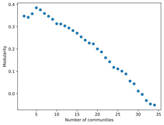
Plot modularity vs community size

import matplotlib.pyplot as plt
plt.plot(NP,MOD,"o")
plt.ylabel('Modularity')
plt.xlabel('Number of communities')
Text(0.5, 0, 'Number of communities')

Visualize Max modularity partition

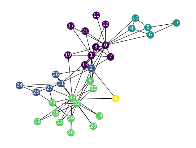
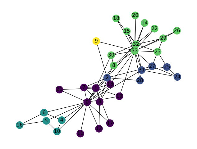
  • From the curve we can see the maximum modularity occurs with FIVE partitions
for partition in partition_sequence:
    if len(partition) == 5:
        five_cluster_partition = partition
        break

print("NETWORK-X SOLUTION:",five_cluster_partition)
plot_partition(K,five_cluster_partition)
NETWORK-X SOLUTION: ({0, 1, 3, 7, 11, 12, 13, 17, 19, 21}, {2, 24, 25, 27, 28, 31}, {4, 5, 6, 10, 16}, {32, 33, 8, 14, 15, 18, 20, 22, 23, 26, 29, 30}, {9})

Visualize partition with two communities

  • Let’s isolate the partition from the partition_sequence with only TWO communities
for partition in partition_sequence:
    if len(partition) == 2:
        two_cluster_partition = partition
        break

plot_partition(K,two_cluster_partition)

Compare with ground truth

print(two_cluster_partition)
print("MODULARITY: ", nx.community.quality.modularity(K, two_cluster_partition))

print("\n",empirical_partition)
print("MODULARITY: ", nx.community.quality.modularity(K, empirical_partition))
({0, 1, 3, 4, 5, 6, 7, 10, 11, 12, 13, 16, 17, 19, 21}, {2, 8, 9, 14, 15, 18, 20, 22, 23, 24, 25, 26, 27, 28, 29, 30, 31, 32, 33})
MODULARITY:  0.3476602762317048

 [{0, 1, 2, 3, 4, 5, 6, 7, 8, 10, 11, 12, 13, 16, 17, 19, 21}, {32, 33, 9, 14, 15, 18, 20, 22, 23, 24, 25, 26, 27, 28, 29, 30, 31}]
MODULARITY:  0.39143756676224206
  • Pretty good – comparable to the ground truth community labels.
  • We can see that the predicted community labels are pretty accurate, only differing on a couple nodes that, visually, seem like they could plausibly belong to either group.
  • Zachary’s original paper even explains the practical considerations of one of these mis-predicted nodes: student 8 was very near receiving his black belt from Mr. Hi and thus did not want to leave the group even though several of his friends did.

Girvan-Newman algorithm (optional)

Coding the algorithm “from scratch”

Summary

  • Our task in this part will be to implement the Girvan-Newman clustering algorithm.

  • Since NetworkX can do the heavy lifting for us – computing betweenness centrality – the code part of the task is relatively straightforward.

  • Most of our effort here is spent interpreting and explaining intermediate results.

  • Recall from the text the Girvan-Newman clustering algorithm:

  1. Create a partition sequence
  2. Calculate the betweenness centrality for all links.
  3. Remove the link with largest betweenness and create a partition using connected components.
  4. Recalculate the betweenness centrality of the links of the resulting graph.
  5. Repeat from step B until no links remain.
  6. Evaluate each partition in the sequence and choose the one with the highest modularity.
  • During this process, the number of connected components in the graph will increase monotonically as clusters are broken up. Since we are removing one link at a time, the number of connected components can increase by at most one between steps in the sequence – it’s not possible for a single edge to connect more than two nodes, and thus components.
  • We hope that the resulting partition of the graph will approximate its underlying community structure. We’ll use the Karate Club graph here because we know the ground-truth community labels and can compare the result obtained from the algorithm.

Setup

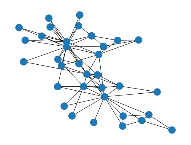
G = nx.karate_club_graph()
nx.draw(G)

Create a partition sequence

Create a partition using connected components

This one is almost a gimme because the nx.connected_components() function gives us almost exactly what we want:

nx.connected_components(G)
<generator object connected_components at 0x11296a730>

We just have to remember to ask for it in a list:

list(nx.connected_components(G))
[{0,
  1,
  2,
  3,
  4,
  5,
  6,
  7,
  8,
  9,
  10,
  11,
  12,
  13,
  14,
  15,
  16,
  17,
  18,
  19,
  20,
  21,
  22,
  23,
  24,
  25,
  26,
  27,
  28,
  29,
  30,
  31,
  32,
  33}]

Remember: a partition is a list of sets where every node is in exactly one of these sets. This is just what we have here, although it’s a bit boring since we’ve only removed one edge and so there is still one connected component. If you like, you can try running the previous two cells a few times until you have more than one connected component so you can see what that looks like.

Note that this feature whereby the connected components correspond exactly to our putative community labels is particular to the Girvan-Newman algorithm: other clustering algorithms may use different ways of generating their partitions.

Recalculate the betweenness centrality

Evaluate the modularity

Do this for each partition in the sequence

We now have a sequence of partitions and a function to calculate the modularity of a partition. This is a great time to use a list comprehension!

G = nx.karate_club_graph()
modularity_sequence = [modularity(G, p) for p in partition_sequence]
print(modularity_sequence)
231
231
231
231
231
231
231
231
231
231
231
231
231
231
231
231
231
231
231
231
231
231
231
231
231
231
231
231
231
231
231
231
231
231
231
231
231
231
231
231
231
231
231
231
231
231
231
231
231
231
231
231
231
231
231
231
231
231
231
231
231
231
231
231
231
231
231
231
231
231
231
231
231
231
231
231
231
231
[0.0, 0.0, 0.0, 0.0, 0.0, 0.0, 0.0, 0.0, 0.0, 0.0, 0.34766027623170476, 0.34766027623170476, 0.34766027623170476, 0.3423192968647515, 0.3423192968647515, 0.3423192968647515, 0.3423192968647515, 0.3580611307884035, 0.3580611307884035, 0.3580611307884035, 0.3580611307884035, 0.3580611307884035, 0.3580611307884035, 0.38497217068645645, 0.37578006409175246, 0.37578006409175246, 0.3594760218136842, 0.3594760218136842, 0.3470699574595679, 0.3470699574595679, 0.333249002080171, 0.333249002080171, 0.3134405277262421, 0.3134405277262421, 0.3122598901819681, 0.3122598901819681, 0.3036862127771219, 0.3036862127771219, 0.2942973332583722, 0.2942973332583722, 0.2827158411573995, 0.2827158411573995, 0.27116245947414774, 0.27116245947414774, 0.2544648713479881, 0.2544648713479881, 0.2397537527407657, 0.2397537527407657, 0.22689792170311643, 0.22299057363992422, 0.22299057363992422, 0.22299057363992422, 0.20056783043796034, 0.20056783043796034, 0.18696238826108955, 0.18696238826108955, 0.18696238826108955, 0.16091340117314143, 0.16091340117314143, 0.16091340117314143, 0.14281029216094152, 0.14281029216094152, 0.11768894885778004, 0.11088622776934466, 0.10076647738985403, 0.08837915331421826, 0.08837915331421826, 0.05623957572009519, 0.04398343359382318, 0.04398343359382318, 0.04398343359382318, 0.011515901126290725, 0.011515901126290725, -0.003504432075860656, -0.031052641442251845, -0.031052641442251845, -0.04655085174565696, -0.05110473941642774]

Modularity plot

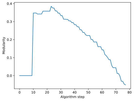
This sequence is then the modularity of the partition at each step in the algorithm. The first several entries in this sequence are effectively zero while there is only one community/component, then it jumps up once there is more than one community. We can use pyplot to visualize this relationship:

import matplotlib.pyplot as plt
plt.plot(modularity_sequence)
plt.ylabel('Modularity')
plt.xlabel('Algorithm step')
Text(0.5, 0, 'Algorithm step')

Visualize partition with highest modularity

Visually, we see a peak in the modularity sequence. This is the partition that maximizes modularity, and thus the output of the algorithm.

  • Write code to isolate the partition with highest modularity.
  • Then plot the resultant partition
max_index=0
for i in range(0,len(modularity_sequence)):
    if(modularity_sequence[i]==max(modularity_sequence)):
        max_index=i
        max_modularity=modularity_sequence[i]

#CHECK 
print(max_index,max_modularity,max(modularity_sequence))
best_partition = partition_sequence[max_index]
23 0.38497217068645645 0.38497217068645645
print(best_partition)
[{0, 1, 3, 7, 11, 12, 13, 17, 19, 21}, {2, 24, 25, 27, 28, 31}, {4, 5, 6, 10, 16}, {32, 33, 8, 14, 15, 18, 20, 22, 23, 26, 29, 30}, {9}]
plot_partition(K,best_partition)

Note

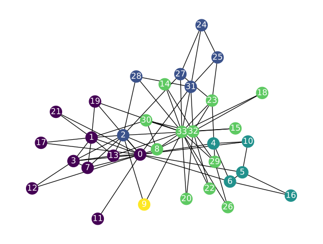
  • Interesting! The partition of the karate club graph with highest modularity actually has five components!
  • Let’s visualize them, using our code for partition maps we wrote back at the beginning of this tutorial:
def create_partition_map(partition):
    partition_map = {}
    for idx, cluster_nodes in enumerate(partition):
        for node in cluster_nodes:
            partition_map[node] = idx
    return partition_map
best_partition_map = create_partition_map(best_partition)

node_colors = [best_partition_map[n] for n in G.nodes()]
nx.draw(G, with_labels=True, node_color=node_colors)

Exactly how good is this five-community clustering?

nx.community.quality.modularity(G, best_partition)
0.3849721706864564

It’s higher than the “ground truth” communities we evaluated in section 3, which is a good sign, but for the specific problem of trying to predict the post-split community membership, a clustering into five groups is useless to us.

Get the best partition with a given number of communities

One of the most useful parts of the Girvan-Newman algorithm is that it is also useful when we have a specific number of clusters we want.

In this case, we know the karate club split into two groups, so let’s get the partition in the sequence with two components:

Aside

The astute reader might note that there may be several two-cluster partitions in the partition sequence we generated. We assert the following to be true:

  1. For every integer 1 to N, the number of nodes, there is a partition in the sequence with that number of clusters
  2. Every partition in the sequence with the same number of clusters is the same

Proving these is left as an exercise to the reader, but as a consequence of these being true, optimized implementations of Girvan-Newman clustering will only store one partition for each number of clusters. This is how the implementation in NetworkX works, only providing one partition for each number of communities greater than one.