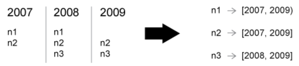
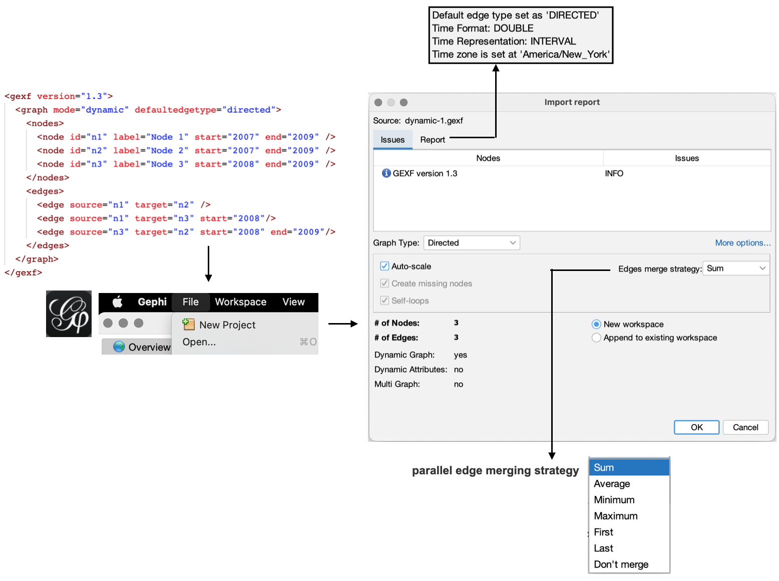
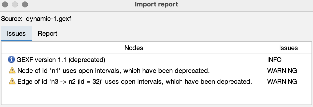
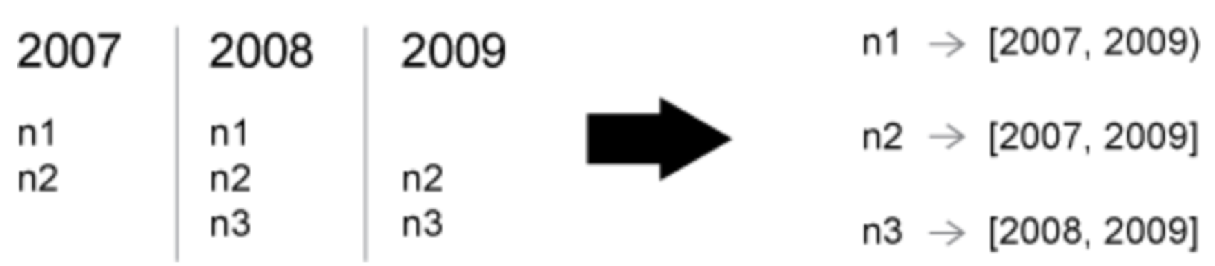
We use the Data Laboratory to see how intervals are created for each node or edge.
When the network is longitudinal, a Time Interval column is present that shows when the interval is present in the graph.
You can visualize this by clicking the checkbox next to ‘Time intervals as graphics’ in the Configuration tab of the Data Laboratory.
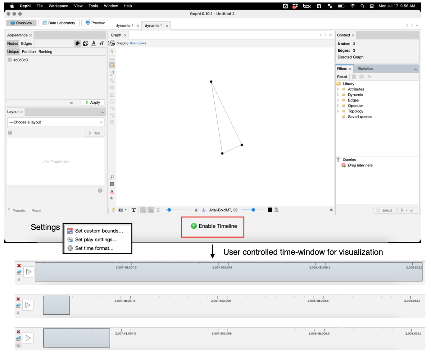
Sliding time window
You can “observe” phenomena over different time-windows in Gephi
This is controlled by the user by varying the size of the blue box
After enabling the timeline, be sure to adjust the size of the window of the sliding filter of your timeline, otherwise you will receive an error stating that Gephi “cannot animate timeline without an animation interval.”
Updating Gephi calculations
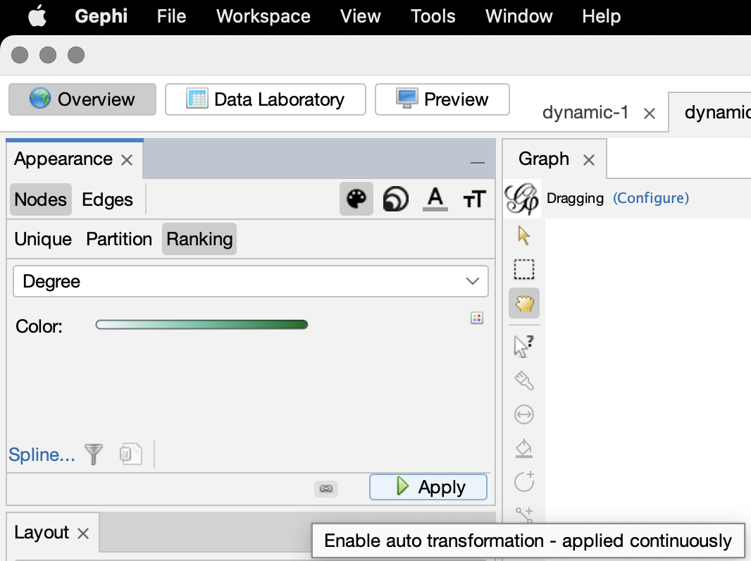
As we’ve seen, Gephi can do various internal calculations (e.g. degree)
If you want these to update dynamically, then you need to use the following button
Run Gephi demo!
Storing dynamic network attributes
The previous exampled showed a variable network topology over time, where nodes and edges are added or remove.
Now let’s see how to represent values changing over time, for example Price.
The attribute definition is the same as for a static GEXF, but the way the values are written has changed.
To represent several values over time, the idea is to repeat the same attvalue for each period, with the same for but with different values and start/end
It’s not mandatory to set a value everywhere, in case of missing the default value is used
For the node ‘n2’, the value ‘12’ starts in 2008 and no end period is specified. That gives the interval [2008, +infinity] which means the value remains ‘12’ in 2009 and after.
The GEXF specifications, including dynamics attributes are available in the GEXF Primer.
Dynamic weight
Normally an edge’s weight is directly defined in the edge element with a particular value.
Defining a dynamic weight attribute overrides this value and provides dynamic weight support.
The rule is to define an edge attribute with the weight keyword for identifier.
Then, use multiple ‘attvalue’ like explained above to set different values over time.
Graph with 2 nodes and 0 edges
-1
-2
{0: 100, 1: -2}
{1: -2}
NetworkX: Dynamic structure
In many ways, NetworkX is designed explicitly for static graphs
Therefore, it takes some hacking to generate a dynamic graph stored in GEXF
Alternatively, You can always create a series of snapshots as well
import networkx as nx # CREATE GRAPH WITH ATTRIBUTESG1=nx.Graph()G1.add_node(0)G1.nodes[0]["start"]=2007G1.nodes[0]["end"]=2008G1.add_node(1)G1.nodes[1]["start"]=2007G1.nodes[1]["end"]=2010G1.add_node(2)G1.nodes[2]["start"]=2007G1.nodes[2]["end"]=2009G1.add_edge(0,1)G1.edges[0,1]["start"]=2007G1.edges[0,1]["end"]=2009nx.write_gexf(G1, "data/dynamic-4.gexf")
DyNetx (optional)
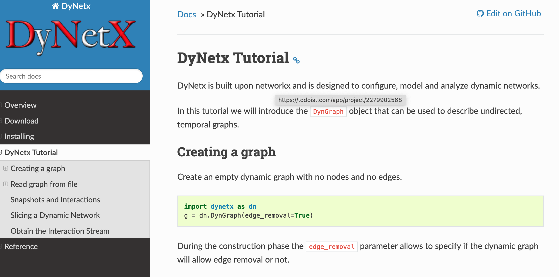
DyNetx is built upon networkx and is designed to configure. model and analyze dynamic networks.
Install: python -m pip install dynetx
Ovito
Lab demonstration: Part-2
Dynamic network visualization with Ovito.
Better suited for LARGE dynamic Networks stored with a snapshot format
Overview
Summary: OVITO is a scientific visualization and data analysis tool for atomistic and other particle-based models.
It helps researchs gain meaningful insights from numerical simulation results.
OVITO can visualize temporal dynamics of large systems of connected data-points (i.e. nodes and edges), in a highly computationally efficient fashion.
The typical use case is for physics applications studying large systems of atoms (up to tens of millions), output from either quantum or classical atomic simulations .
However, it can be “hi-jacked” and used as a more general visualizer for showing data in up to six dimensions.
3 positions x,y,z, 1 color, 1 size, 1 time-dimension, along with particle inter-connectivity (bonds).
Generally you can think of it as an advanced visualization tool for plotting time dependent collections of points in 2D or 3D space (i.e. trajectories)
2D: \(\mathbf{r}_i(t)=(x_i(t),y_i(t))\)
3D: \(\mathbf{r}_i(t)=(x_i(t),y_i(t),z_i(t))\)
IMPORTANT: Often these x,y,z points refer to the dimensions in physical space, however, they don’t have to. They can be any abstract vector of three related data points, for example the first three principle components obtained from running PCA on some dataset.
OVITO: Download
Download: The software is being used across various research disciplines and has served as a valuable scientific tool in more than 7,600 research studies so far (~5 new publications per day).
For professional scientists and academic research groups we offer our powerful OVITO Pro product, which includes an extended analysis tool-set, visualization capabilities and automation functions (Python integration).
Ovito: Versions
The basic community edition is available free of charge under an open source license
NOTE: USE THE FREE ONE .. DON’T PAY FOR THE ADVANCED VERSION.
For this class, the free basic version will be sufficient
OVITO input
Timestep: This represents what iteration of the time loop the snapshot if based on
Box: The software also needs the upper and lower bounds for the x,y,z dimensions.
These define a rectangular (or cubic) “box” where the nodes live.
This box can be
periodic, i.e. a particle loops around to the other-side of the simulation box when it steps outside.
Fixed: i.e a particle “bounces” off the side of the simulation box when it hits the edge and is reflected back inside.
OPTIONAL: additional attributes (size, energy ,etc)
File format
OVITO accepts many different file formats.
One common type is the “LAMMPS” dump format which we will use today.
The following shows examples of the format.
ASIDE: The “Large-scale Atomic/Molecular Massively Parallel Simulator” (LAMMPS) is a molecular dynamics program from Sandia National Laboratories. LAMMPS makes use of the Message Passing Interface (MPI) for parallel communication and is free and open-source software, distributed under the terms of the GNU General Public License.
File format: Node information
We can store nodes, and associated node-attributes in the following formate
In this example the box is cubic (Lx=Ly=Lz=20), however, it could easily be generalized to work with rectangular boxes as well
ITEM: TIMESTEP
1
ITEM: NUMBER OF ATOMS
3
ITEM: BOX BOUNDS ff ff ff
0.0 20.0
0.0 20.0
0.0 20.0
ITEM: ATOMS id x y z type v1
0 6.9153 12.0049 12.6545 1.0 2.0
1 9.3336 0.0 7.6789 1.0 4.0
2 3.3336 0.0 5.6789 1.0 4.0
File format: Edge information
We can store edges (bonds), and associated node-attributes in the following formate
For our purposes only the 3rd and 4rd columns matter.
These columns define the edge list for the system. So the line, 0 1 0 1 1.0 1.0 represents an edge from point 0 to point 1.
import osimport numpy as npimport matplotlib.pyplot as pltimport shutilfrom string import Templateimport networkx as nxfrom IPython.display import Image,Video,HTML
Create a function to delete a folder if it exists, and then create a new folder.
#WARNING: THIS FUNCTION WILL DELETE AND RECREATE THE SPECIFIED FOLDERdef create_folder(out_dir_path):if(os.path.exists(out_dir_path)): shutil.rmtree(out_dir_path) os.mkdir(out_dir_path)
Create a folder names “results-1” to store our snapshots
I wrote the following function for writing data into the “LAMMPS” dump format, which can then be visualized in OVITO.
Currently, it is coded for a cubic simulation box. The code could easily be generalized to the case of a rectangular box.
However, cubic boxes will suffice for our purposes.
import numpy as npfrom string import Template#FUNCTION TO WRITE SNAPSHOT FILES FOR OVITOdef write_ovito_snapshot(L,X,t,file_path,E=[],auto_rescale=False): xyz_min=0 xyz_max=Lif(auto_rescale):#SHIFT TO ORIGIN X[:,0]=X[:,0]-np.min(X[:,0]) X[:,1]=X[:,1]-np.min(X[:,1]) X[:,2]=X[:,2]-np.min(X[:,2])#OPTIONALLY RE-SCALE THE BOX AND POSITIONS SO L~2N scale_factor=2*X.shape[0] X[:,0:3]=scale_factor*X[:,0:3]/(np.max(X[:,0:3])-np.min(X[:,0:3]))#REDEFINE BOX xyz_min=np.min(X[:,0:3]) xyz_max=np.max(X[:,0:3])#STRING TEMPLATE TO BUILD REQUIRED FILE FORMAT my_template = Template("""ITEM: TIMESTEP$tITEM: NUMBER OF ATOMS$NITEM: BOX BOUNDS ff ff ff$Lmin $Lmax$Lmin $Lmax$Lmin $Lmax$INFO""" )#BUILD HEADER INFO="ITEM: ATOMS id x y z type"if(X.shape[1]>4): k=1for i inrange(4,X.shape[1]): INFO+=" v"+str(k); k+=1 INFO+="\n"#LOOP OVER ROWSfor i inrange(0,X.shape[0]):#LOOP OVER COLUMNS INFO+=str(i)+" "for j inrange(0,X.shape[1]): INFO+=str(round(X[i,j],4))+" " INFO+="\n"#POPULATE TEMPLATE out=my_template.substitute({'t' : t,'Lmin' : xyz_min,'Lmax' : xyz_max,'INFO' : INFO,'N' : X.shape[0] } )#print(out)# #SAVE SNAPSHOTwithopen(output_folder+"/"+str(t)+'.dump', 'w') as f: f.write(out)#STRING TEMPLATE TO BUILD REQUIRED FILE FORMAT my_template = Template("""ITEM: TIMESTEP$tITEM: NUMBER OF ENTRIES$NITEM: BOX BOUNDS ff ff ff$Lmin $Lmax$Lmin $Lmax$Lmin $LmaxITEM: ENTRIES index c_1[1] c_1[2] c_1[3] c_2[1] c_2[2] $INFO""" )if(len(E)>0):#LOOP OVER ROWS INFO=""for i inrange(0,E.shape[0]): INFO+=str(i)+" 1 "+str(E[i,0])+" "+str(E[i,1])+" 1.0 1.0 \n" out=my_template.substitute({'t' : t,'Lmin' : xyz_min,'Lmax' : xyz_max,'INFO' : INFO,'N' : E.shape[0] } )#print(out)withopen(output_folder+"/"+str(t)+'.bond.dump', 'w') as f: f.write(out)
Utility function details
L = cubic box length
t = current time step
output_dir_path=path to the output folder to save the snapshot file
MINIMUM INPUT:
X = np.array with positions, types
X = [[x0,y0,z0,type1],[x1,y1,z1,type2] … ]
The “type” is an integer node attribute which specifies the particle type, for example, (Ag=1, Cu=2) or (Democrat=1, Republican=2)
Type should start from 1 and be consecutively defined for each type(1,2,3 …)
OPTIONAL: You can add more particle (node) attributes at the end
X = [[x0,y0,z0,type1,v01,v02 … ],[x1,y1,z1,type2,v11,v12] … ]
Where vij is the jth additional attribute of particles i
OPTIONAL: E=edge list for defining bonds (edges) [[0,1],[1,2]]
The X numpy array stores the node information.
Where the node-id (0,1, 2) is encoded in the row-index of the numpy array (row-0 = node-0 info), (row-1 = node-1 info) … etc.
The edge [0,1] means that there is an edge from node-0 to node-1.
These are stored in a numpy array E representing the edge list E=np.array([[01],[0,2]).
Ovito basics: video
Example-1: Simple network
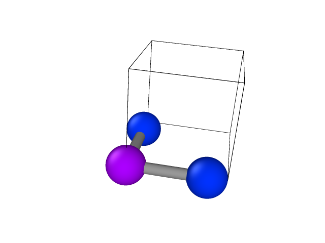
Here we create a numpy array with 3 particles, with two different types, located in a triangle, with bonds from [0,1] and [0,2], situated inside a 5x5x5x box
We use the function above to save the system to a snapshot file, use timestep=t=1
NOTE: This will overwrite the previous OVITO snapshot files
Starting from the configuration in “assignment-1”
Write a time loop that makes the particles execute a random walk, i.e at each timestep
(x –> x+R1, y –> y+R2, z –> z+R3) where R1,R2,R3 are random numbers
Run 100 iterations of the loop, save each iteration to a snapshot
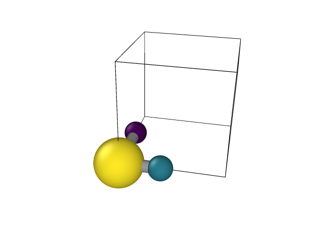
Open OVITO and generate the gif shown below
Make sure under “search pattern” you click “auto-generate” for both particles and bonds, this will recognize 1.dump and 2.dump … as the first and second frames.
L=5#cubic box sizet=1X=np.array([[0.,0,0,2],[0,4,0,1],[4,0,0,1]])E=np.array([[0,1],[0,2]])dx=0.1# Image("media/01.png")#TIME LOOPSfor t inrange(1,100):#LOOP OVER PARTICLES for i inrange(0,X.shape[0]):for j inrange(0,3): X[i,j]=X[i,j]+np.random.uniform(-dx,dx,1)[0] write_ovito_snapshot(L,X,t,output_folder,E)Image("media/03.gif")
<IPython.core.display.Image object>
References
1.
Menczer, F., Fortunato, S. & Davis, C. A. A first course in network science. (Cambridge University Press, 2020).