A generative, inferential view of community structure: assume the network was produced by hidden groups, then work backwards to recover them.
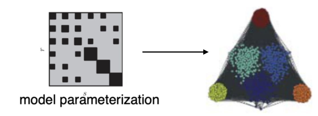
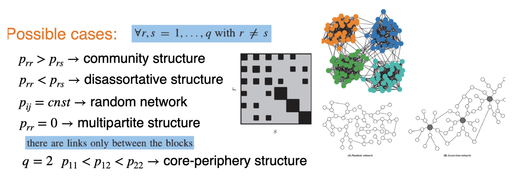
Most widely adopted models for building networks with communities
Motivation
Generative Models in Community Structure
Generative Models: Aim to explain how observed data could be generated by underlying processes.
Purpose: Provide insights into the formation and evolution of communities within networks.
Applications: Useful in social networks, biological systems, and information networks to identify functional groups.
Benefits:
Enhance understanding of complex systems.
Predict future interactions or changes in the network.
Inform strategies for intervention or optimization.
Two philosophies of community detection
1. Descriptive / optimization: “find groups that score well.” - Pick a quality function (modularity, cut ratio, conductance) and optimize it. - Fast and intuitive, but the objective defines what a community is, and can suffer from resolution limits and overfitting to noise.
2. Generative / inferential: “assume the data came from a model with hidden groups, then fit it.” - Write down a probability model that generates networks with communities, - then invert it to recover the groups.
Stochastic Block Models (SBMs) are the canonical generative approach.
Why bother with a generative model?
Principled: communities are parameters to estimate, not arxtifacts of a scoring rule.
Uncertainty & model selection: how many communities?
General structure: not just assortative “clumps”: also bipartite, core–periphery, hierarchical patterns.
A ground-truth generator: SBMs are the standard benchmark for testing any detection algorithm.
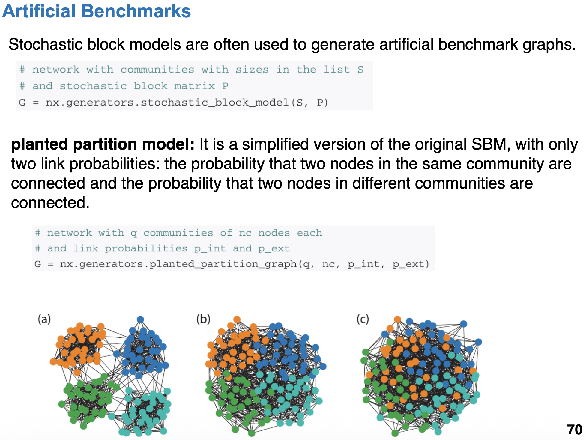
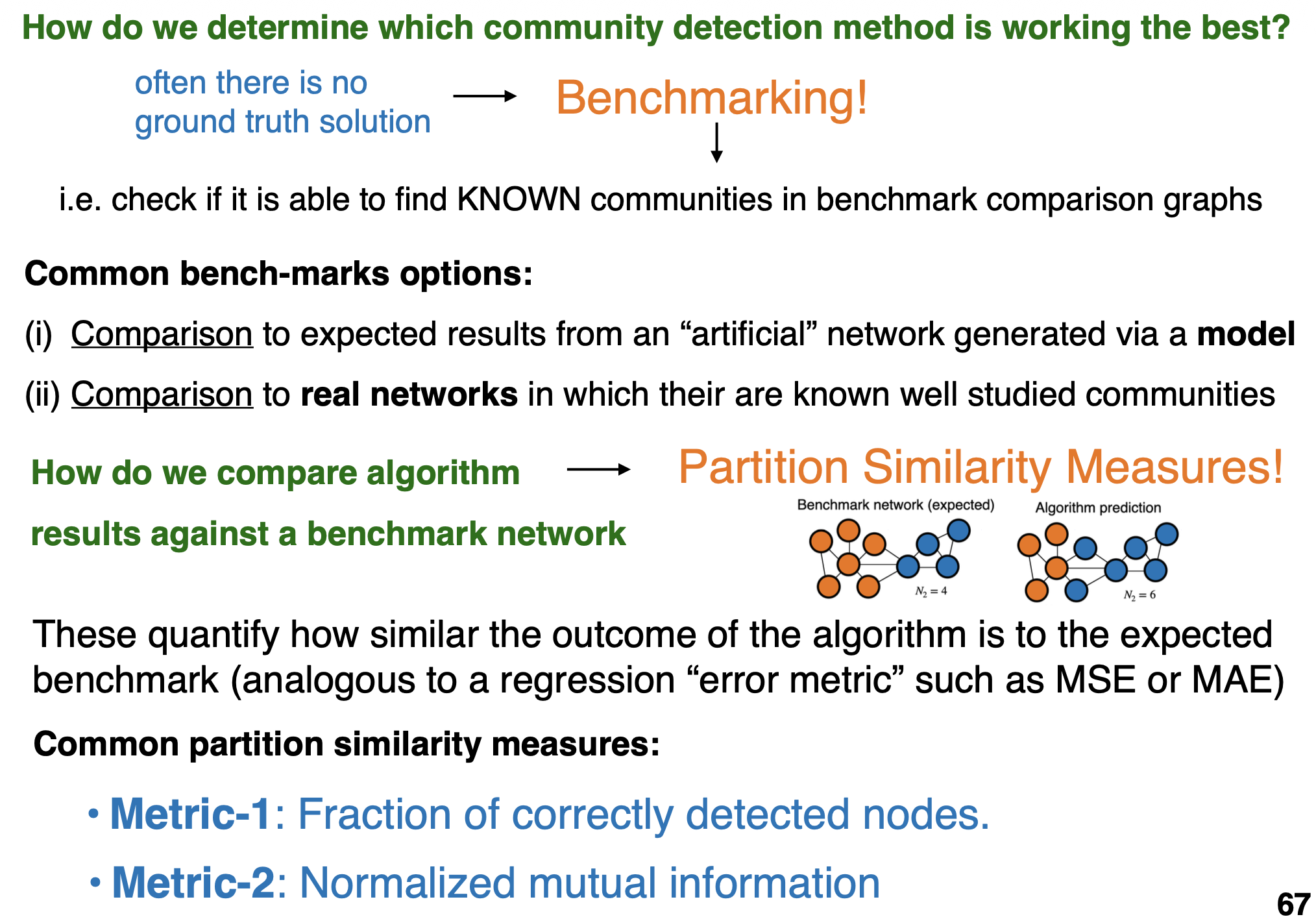
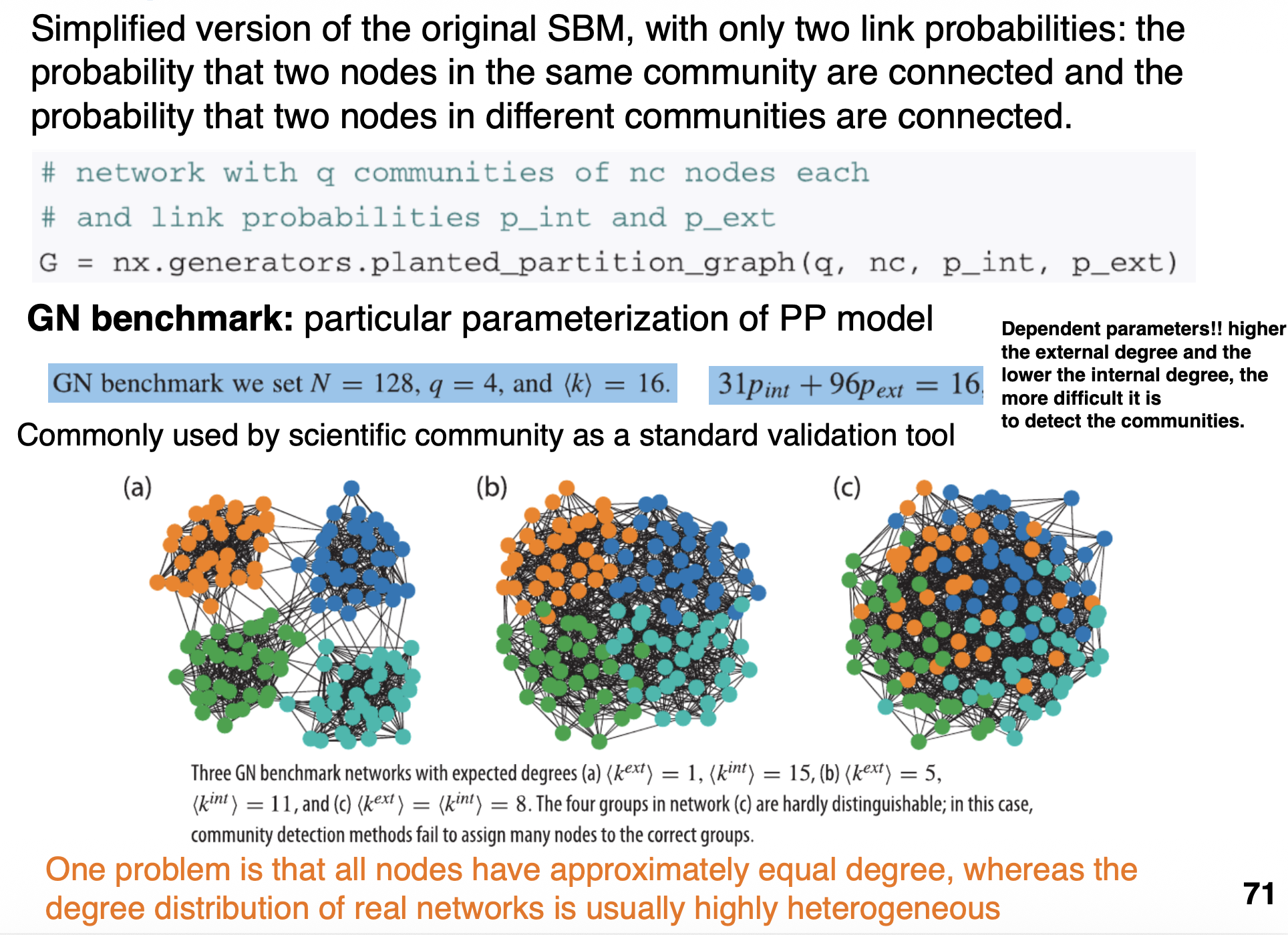
Generative models serve as artificial bench marks
Partion models also serve as evaluation benchmarks
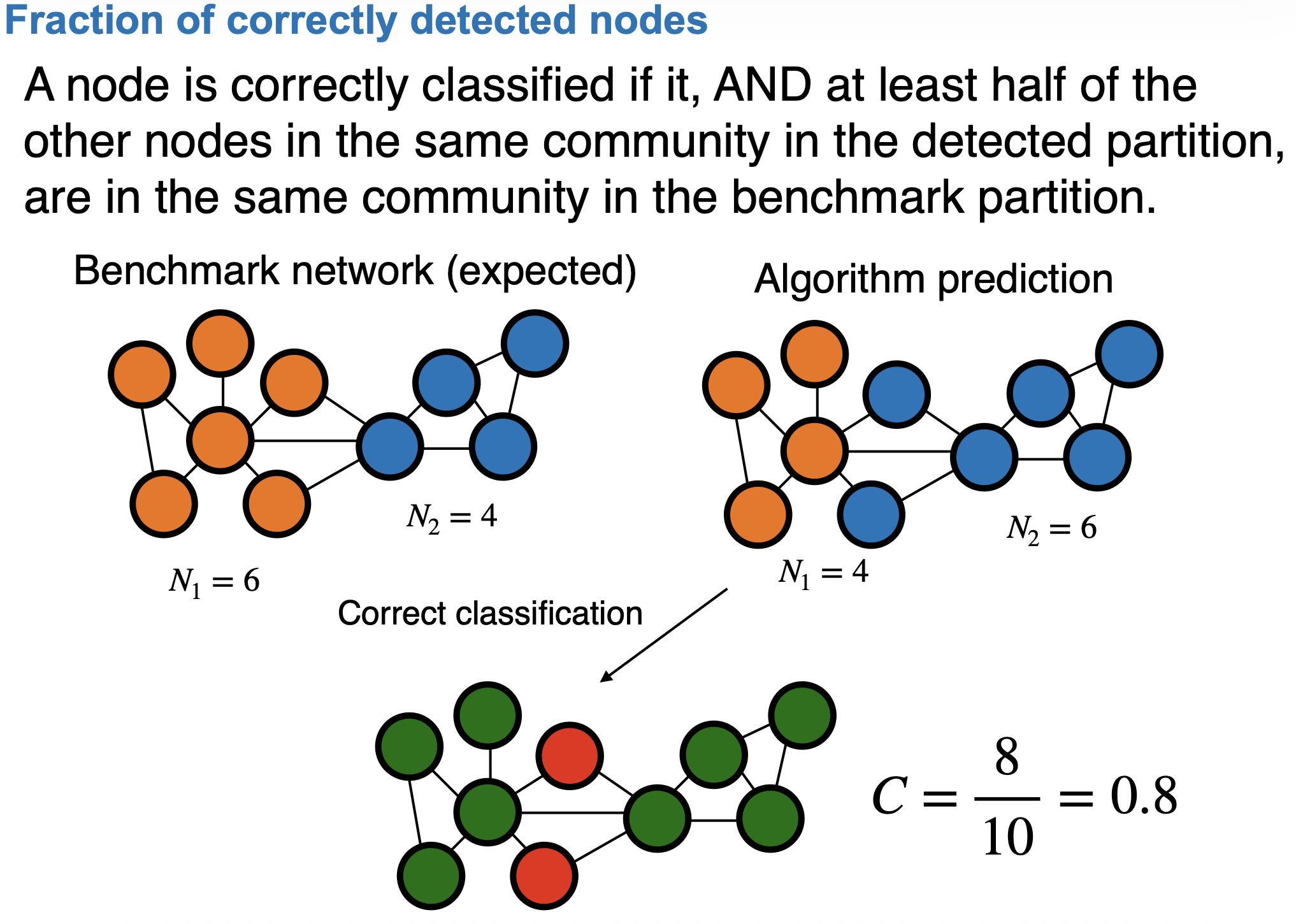
Validation metric-1: Fraction of correctly classified nodes
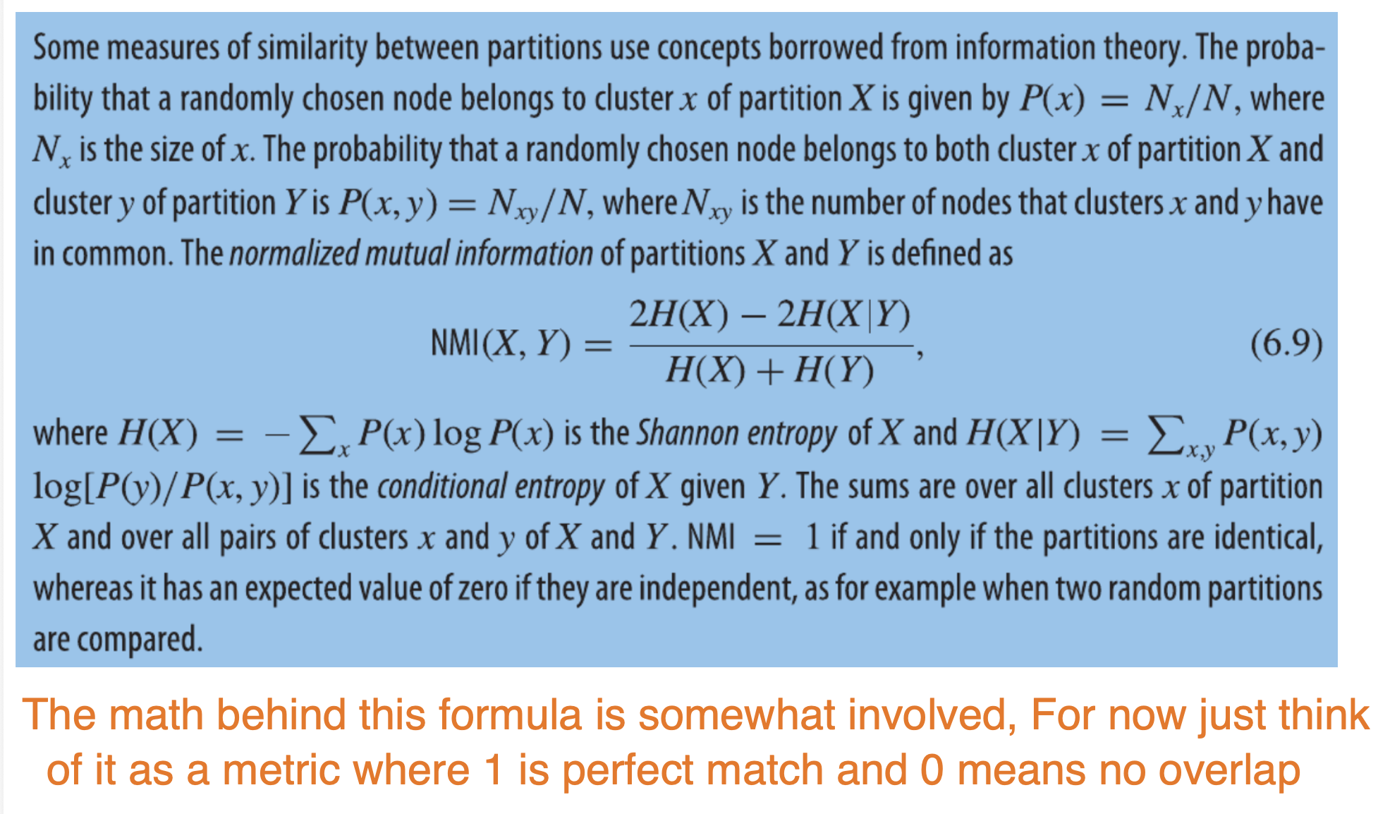
Validation metric-2: Normalized mutual information
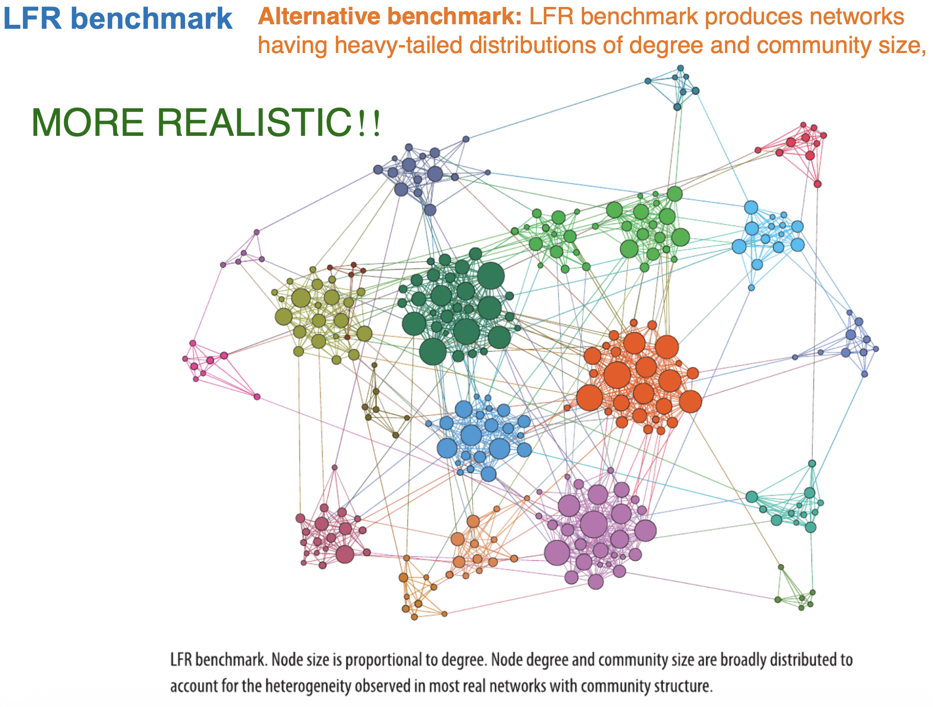
LFR Benchmark
The LFR benchmark is a widely-used artificial test network that realistically imitates properties of real-world networks, including heterogeneous node degrees and community sizes, to evaluate community detection algorithms.
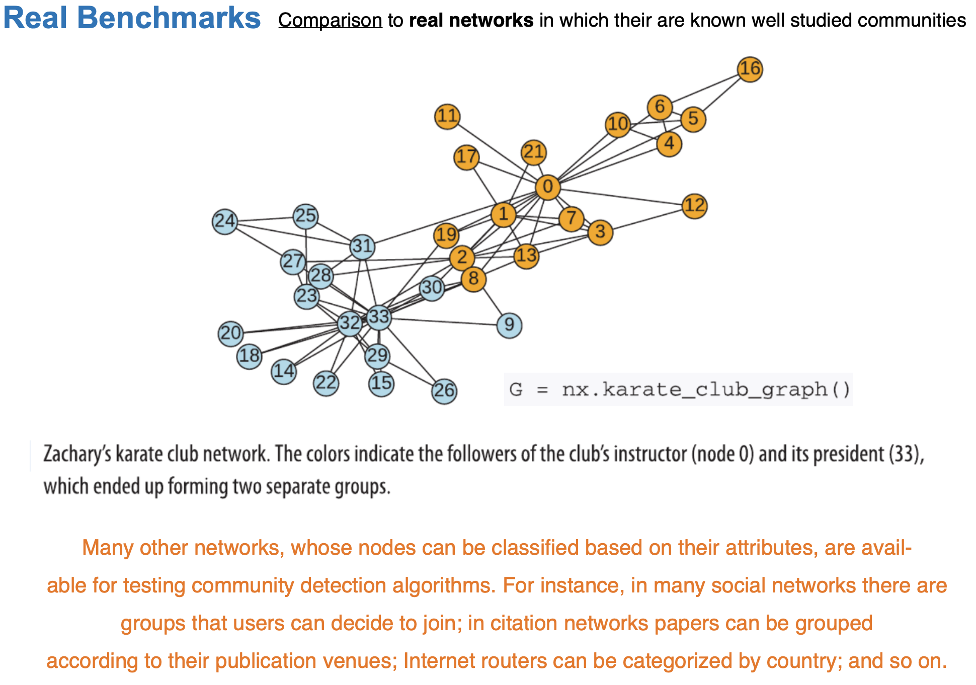
Real world benchmarks: E.g. Zachary’s Karate Club
Stochastic Block Models
The core idea of a block model
Every node belongs to a hidden block (group). The probability that two nodes connect depends only on their blocks: not on their individual identities.
Nodes in the same block are stochastically equivalent: swap two of them and the statistics of the graph are unchanged.
Analogy. In a university, whether two people connect depends mostly on their role: student, faculty, staff: and on how those roles tend to interact, not on the specific individuals.
General idea:
nodes are divided into various groups where the probability that two nodes are connected is dependent on group memberships
A network with \(N\) nodes is partitioned into \(q\) groups.
Each node \(i\) belongs to a group \(g_i\).
The connection probability between nodes \(i\) and \(j\) depends only on their group memberships: \(P(i \leftrightarrow j) = p_{g_i g_j}\).
All node pairs from groups \(g_1\) and \(g_2\) share the same connection probability \(p_{g_1 g_2}\).
These probabilities form a \(q \times q\)stochastic block matrix.
For undirected graphs, the matrix is symmetric; for directed graphs, it may be asymmetric.
Limitation: need to specify the number of groups beforehand
Building an SBM in NetworkX
nx.stochastic_block_model(sizes, p, seed=...)
sizes: list of block sizes; sets \(n\)and the partition. e.g. [30, 25, 20].
p: a \(k\times k\) list-of-lists; p[r][s] is the edge probability between blocks \(r\) and \(s\) (symmetric for an undirected graph). This is the matrix \(B\).
NetworkX tags every node with its block id in the "block" attribute.
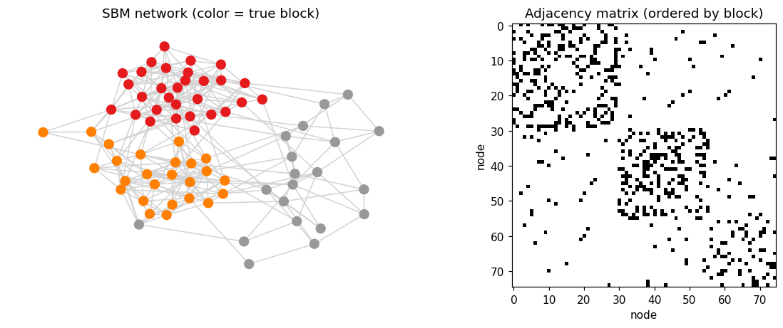
import numpy as npimport networkx as nximport matplotlib.pyplot as pltplt.rcParams["figure.dpi"] =110# crisp inline figuresSEED =42# reproducibility everywhere# --- An assortative SBM with three communities ---------------------------sizes = [30, 25, 20] # 3 blocks -> n = 75 nodes# Block matrix B: large diagonal (dense within), small off-diagonal (sparse between).# Must be symmetric because the graph is undirected.p = [[0.25, 0.02, 0.02], [0.02, 0.30, 0.03], [0.02, 0.03, 0.25]]G = nx.stochastic_block_model(sizes, p, seed=SEED)# Each node carries its ground-truth block id under the 'block' attribute.blocks = [G.nodes[v]["block"] for v in G.nodes()]print(f"{G.number_of_nodes()} nodes, {G.number_of_edges()} edges, {len(sizes)} blocks")
75 nodes, 287 edges, 3 blocks
Interpreting the visualization
The dense squares on the diagonal of the adjacency matrix are the communities.
But this clean block structure only appears because the nodes happen to be ordered by block. Real data arrives in arbitrary order: the whole job of community detection is to find the permutation that reveals these blocks.
# --- Two complementary views: the network, and its adjacency matrix -------fig, (ax1, ax2) = plt.subplots(1, 2, figsize=(11, 4.3))pos = nx.spring_layout(G, seed=SEED) # force layout separates dense groupsnx.draw_networkx(G, pos, node_color=blocks, cmap=plt.cm.Set1, node_size=70, with_labels=False, edge_color="lightgray", ax=ax1)ax1.set_title("SBM network (color = true block)"); ax1.axis("off")# Nodes are stored in block order, so the adjacency matrix shows dense# diagonal blocks -- the visual signature of assortative community structure.A = nx.to_numpy_array(G)ax2.imshow(A, cmap="Greys", interpolation="nearest")ax2.set_title("Adjacency matrix (ordered by block)")ax2.set_xlabel("node"); ax2.set_ylabel("node")plt.tight_layout(); plt.show()
SBM: Meaning of the parameters
Planted Partition Model
The Planted Partition Model (PPM)
The simplest, most-studied SBM: also called the symmetric SBM.
All communities are equal-sized and interchangeable, and \(B\) has just two distinct values:
Simplified probability matrix: \(P_{in}\) for intra-block, \(P_{out}\) for inter-block.
\[B_{rs} = \begin{cases} p_{\text{in}} & r = s \quad(\text{within a community})\\[2pt] p_{\text{out}} & r \neq s \quad(\text{between communities}) \end{cases}\]
Two knobs only: \(p_{\text{in}}\) and \(p_{\text{out}}\).
k: nodes per community (equal sizes) → total \(n = l \cdot k\).
p_in: within-community edge probability.
p_out: between-community edge probability.
Note that \(p_{in}\) and \(p_{out}\) don’t need to sum to 1:
Need unequal community sizes? Use the sibling nx.random_partition_graph(sizes, p_in, p_out, seed=...), where sizes is a list like the SBM’s.
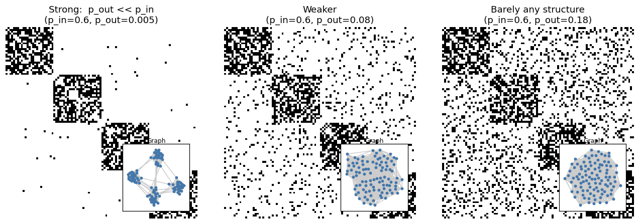
# --- How structure fades as p_out approaches p_in ------------------------def ppm_adjacency(l, k, p_in, p_out, seed=1):"Planted-partition graph -> adjacency matrix (nodes ordered by community)." G = nx.planted_partition_graph(l, k, p_in, p_out, seed=seed)return nx.to_numpy_array(G)l, k =4, 25# 4 communities x 25 nodes = 100 nodesp_in =0.6fig, axes = plt.subplots(1, 3, figsize=(12, 4))settings = [(0.005, "Strong: p_out << p_in"), (0.08, "Weaker"), (0.18, "Barely any structure")]for ax, (p_out, label) inzip(axes, settings):# Show adjacency matrix adj = ppm_adjacency(l, k, p_in, p_out) ax.imshow(adj, cmap="Greys") ax.set_title(f"{label}\n(p_in={p_in}, p_out={p_out})") ax.axis("off")# Visualize the generated graph in a small insetfrom mpl_toolkits.axes_grid1.inset_locator import inset_axes G = nx.planted_partition_graph(l, k, p_in, p_out, seed=1) ax_inset = inset_axes(ax, width="35%", height="35%", loc='lower right', borderpad=1) nx.draw_networkx(G, ax=ax_inset, node_size=8, pos=nx.spring_layout(G, seed=1), with_labels=False, edge_color="#cccccc", node_color="#4477AA") ax_inset.set_xticks([]); ax_inset.set_yticks([]) ax_inset.set_title("Graph", fontsize=8, pad=2)plt.tight_layout(); plt.show()
/var/folders/lc/n91cn5z96ws6f52d25t2rpbh0000gn/T/ipykernel_57595/3035322147.py:32: UserWarning: This figure includes Axes that are not compatible with tight_layout, so results might be incorrect.
  plt.tight_layout(); plt.show()
Limiting case:
As \(p_{\text{out}} \to p_{\text{in}}\) the diagonal blocks wash out and the graph becomes indistinguishable from pure noise (Erdős–Rényi).
This raises a sharp question: is there a point past which the communities are provably impossible to recover: no matter how clever the algorithm?
Inference with Partition Models
Recall: MLE with a Gaussian
The setup. We have data \(x_1,\dots,x_n\) and assume it came from a normal distribution: but we don’t know its mean \(\mu\) or variance \(\sigma^2\). Goal: recover the parameters that best explain the data.
Step 1: Write the likelihood. Each point has density \(f(x_i)=\tfrac{1}{\sqrt{2\pi\sigma^2}}\,e^{-(x_i-\mu)^2/2\sigma^2}\). Assuming independence, multiply:
The takeaway:“which parameters make the observed data most likely?” The answer is just the obvious summary statistics: and this write it → log it → maximize it recipe is exactly what we do for the PPM. The only twist there: one of the parameters (the community labels) is discrete, so that piece needs a search instead of a clean derivative.
We can do a similar thing for the PPM too, but the math is more complicated.
Inference with the PPM: motivation
So far we’ve run the PPM forward: pick \(p_\text{in}, p_\text{out}\), hidden labels \(z\), and generate a network. But with real data we face the reverse problem:
\[\text{we see only } A \;\longrightarrow\; \text{recover the hidden communities } \hat z\]
The network arrives as a scrambled pile of nodes and edges.
Nobody hands us the labels: that’s the whole point.
The key idea: treat the PPM as a hypothesis about how the graph was born, and ask —
“Which assignment of nodes to groups makes the graph we actually see most believable?”
Because the PPM has just two knobs (\(p_\text{in}\) for within-group links, \(p_\text{out}\) for between), this reduces to one intuitive test: find the split that is dense inside and sparse between. That’s a partition where within-group ties look like \(p_\text{in}\) and cross-group ties look like \(p_\text{out}\): with \(p_\text{in} \gg p_\text{out}\).
A good split → the adjacency matrix lights up in dense diagonal blocks.
A bad split → edges scattered everywhere, no block structure.
Inference is simply searching partitions and scoring how believable each one is: turning “find the communities” into a well-posed estimation problem.
Steps of inference with the PPM
The PPM has only two knobs: \(p_\text{in}\) (within-group) and \(p_\text{out}\) (between-group): so recovering communities boils down to one question: which split packs the most edges inside groups?
Step 1: Propose a partition \(z\). A guess at the \(k\) equal-sized communities.
Step 2: Fill in the two knobs for free. Given the split, their best estimates are just the observed densities:
\[\hat p_\text{in} = \frac{\text{edges inside groups}}{\text{pairs inside groups}}, \qquad \hat p_\text{out} = \frac{\text{edges between groups}}{\text{pairs between groups}}.\]
Step 3: Score it. Reward the split for every within-group edge and every between-group gap. A partition scores high exactly when \(\hat p_\text{in} \gg \hat p_\text{out}\): dense inside, sparse between.
Step 4: Improve. Move a node to another group, re-score, keep moves that raise it. Repeat until no move helps.
Step 5: Sanity check. If \(\hat p_\text{in} \approx \hat p_\text{out}\), the “communities” are just noise: recall the detectability threshold: below it, no amount of searching can recover real groups.
Intuition: the whole search is hunting for the split that makes the diagonal blocks of the adjacency matrix as dense as possible and the off-diagonal blocks as empty as possible.
Methods for Finding the best partition
We can’t just test every partition: the number of ways to split \(n\) nodes into groups explodes (the Bell numbers grow faster than exponentially). So we need smart search:
Maximum likelihood: hill-climbing: nudge nodes between blocks, keep the moves that raise the score. Simple, but can get stuck in a local peak.
Bayesian / MCMC: don’t hunt for one “best” answer; sample many plausible ones. Bonus: it infers how many communities \(k\) exist on its own, with a built-in penalty against overfitting (Occam’s razor).
Belief propagation: nodes gossip their best self-guess to their neighbors and update until everyone agrees. Fast, and it pinpoints the exact threshold where detection becomes impossible.
Spectral methods: skip the search: read the groups straight off the top eigenvectors of the matrix (fast linear algebra: ties back to spectral lectures).
Forward model = how the graph was born. Inference = rewinding the tape to recover the hidden groups.
Degree Corrected Stochastic Block Model (DCSBM)
Motivation for DCSBM
Limitation of Standard SBM: The standard Stochastic Block Model (SBM) performs poorly on real networks because it assumes uniform degree distribution, ignoring degree heterogeneity.
Motivation for DCSBM: The Degree-Corrected Stochastic Block Model (DCSBM) addresses this by incorporating actual node degrees, enabling more accurate modeling of networks with variable connectivity.
degree (“high-degree” vs “low-degree”) instead of by genuine community.
Fix. Give each node a propensity \(\theta_i\) so the expected edge rate becomes
\(L_{rs}\): Number of edges between group \(r\) and group \(s\)
\(k_r\), \(k_s\): Sum of degrees of nodes in group \(r\) and \(s\), respectively
Measures how likely it is that the observed network \(G\) was generated from partition \(g\) under the DCSBM.
Greedy Likelihood Maximization Algorithm
Greedy Likelihood Maximization Algorithm:
Initialization: Start with a random division of nodes into \(q\) groups (i.e., a random \(g\)).
Step 1 – Node Reassignment:
For each node, try moving it to a different group to increase (or least decrease) the log-likelihood.
Each node is moved only once per iteration.
Step 2 – Best Partition Selection:
Among all partitions visited in Step 1, select the one with the highest likelihood.
Stopping Criterion:
The algorithm halts when likelihood converges (i.e., no change between successive iterations).
Inference with the DC-SBM:
score every partition, keep the best: but the scoring now accounts for hubs.
Step 0: Precompute (once). Node degrees \(k_i\), and for any grouping, the edge counts \(m_{rs}\) and group degree-sums\(\kappa_r = \sum_{i\in r} k_i\).
Step 1: Propose a partition \(z\). A guess at who’s in which block.
Step 2: Fill in the rest of the recipe for free. The nuisance parameters have closed-form MLEs: no searching needed:
\[\hat\theta_i = \frac{k_i}{\kappa_{z_i}} \quad(\text{node's share of its group}), \qquad \hat\omega_{rs} = m_{rs}.\]
Step 3: Score the partition. Plug those back in; everything collapses to a function of \(z\) alone:
Step 4: Improve. Move a node to a neighboring block, recompute \(\mathcal L\), keep moves that raise it (greedy / agglomerative). Repeat to convergence.
Step 5: Escape local peaks & pick \(k\). Restart from many seeds; or go Bayesian (MCMC over \(z\)) to sample partitions and infer the number of blocks automatically.
Summary of models
SBM = a generative model: edge probability depends only on block membership
The pattern of \(B\) sets the structure: assortative, disassortative, or core–periphery: not just clumps.
PPM = symmetric SBM with two knobs, \(p_{\text{in}}\) and \(p_{\text{out}}\); the field’s standard benchmark.
Detectability threshold: weak communities are provably unrecoverable: a real phase transition.
Detection = inference: invert the generative process via likelihood, Bayes/MCMC, belief propagation, or spectral methods.
DC-SBM makes the model usable on real, heavy-tailed networks.
Extra: PPM Fitting example
Description of what this code does:
Setup: Imports NumPy, NetworkX, Matplotlib; seeds a random generator for reproducibility.
Define the PPM likelihood (ppm_log_likelihood): Given a community assignment z and adjacency matrix A:
Flags every node pair as same-community or different-community (upper triangle only, so each pair counts once).
Counts within-community edges m_in and cross-community edges m_out, plus how many pairs of each type exist.
Sets the fitted probabilities to the observed densities: p_in = m_in / #same-pairs, p_out = m_out / #diff-pairs.
Returns the profile log-likelihood (sum of two Bernoulli-block terms) along with p_in, p_out.
Define the inference objective (score): Returns the log-likelihood only if the split is assortative (p_in > p_out); otherwise −inf. This enforces the “planted” (assortative) assumption and blocks the degenerate degree-based split.
Inference by greedy hill-climbing (infer): For each of 40 random restarts:
Start from a random 2-way labeling.
Sweep over nodes, flipping any node whose reassignment raises the score; repeat sweeps until no flip helps.
Track the best-scoring labeling across all restarts.
Run on Karate Club:
Loads nx.karate_club_graph(), builds A, and reads ground-truth factions from the 'club' node attribute.
Runs infer to get the predicted labels.
Aligns the arbitrary {0,1} labels to the ground truth (flips if agreement < 50%).
Computes accuracy, fitted p_in/p_out, and the misclassified nodes, then prints them.
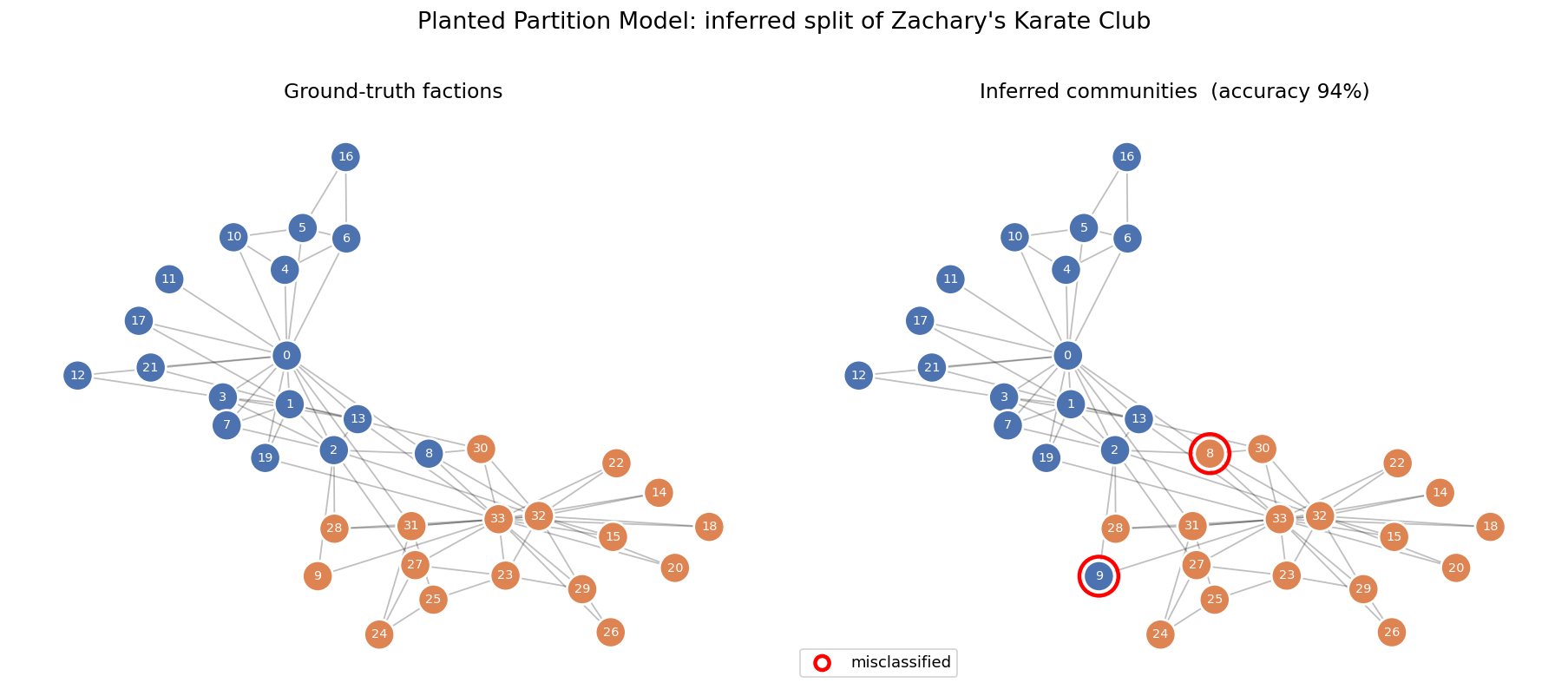
Visualization A: graphs: Draws two side-by-side spring layouts (shared positions): ground-truth factions vs. inferred communities, coloring nodes by community and ringing misclassified nodes in red.
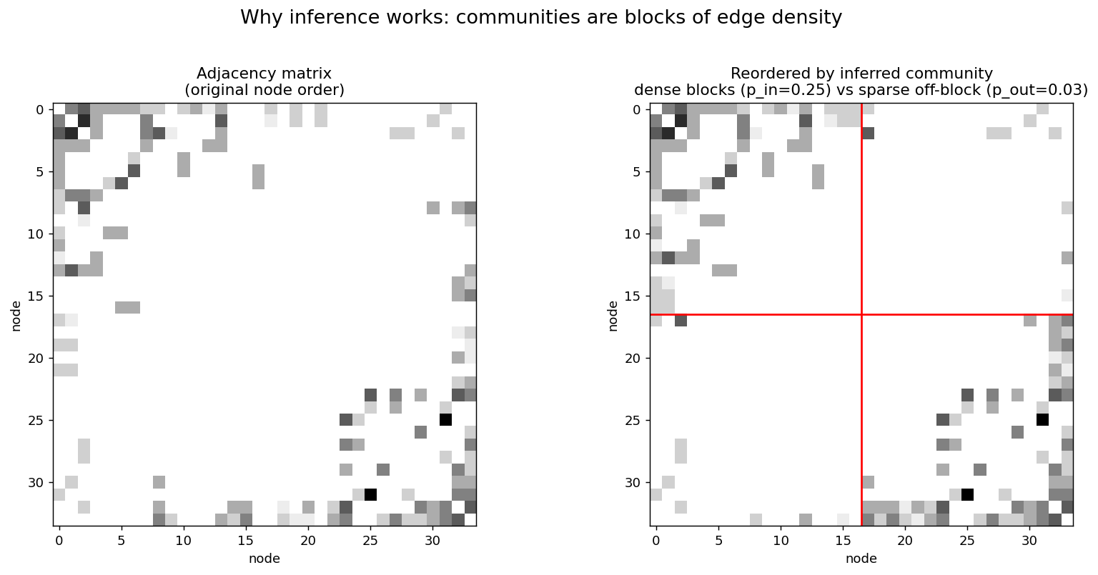
Visualization B: block structure: Shows the adjacency matrix in original order vs. reordered by inferred community, with red lines marking the community boundary to reveal the dense diagonal blocks (p_in) against the sparse off-diagonal block (p_out).
Save: Writes both figures to images/ and prints a confirmation.
One note: the file references an images/ directory for saving (and has a trailing # show the images comment with nothing after it): make sure that folder exists before running, or the savefig calls will error.
Source: Claude
"""Community detection by INFERENCE with the Planted Partition Model (PPM)======================================================================The Planted Partition Model is the simplest Stochastic Block Model: * every node belongs to one of k communities (here k = 2) * two nodes in the SAME community are linked with probability p_in * two nodes in DIFFERENT communities are linked with probability p_out * "planting" communities means the structure is ASSORTATIVE: p_in > p_outDetecting communities "by inference" = find the node->community assignment zthat makes the observed graph MOST PROBABLE under this model (maximumlikelihood). No modularity, no black box -- just the generative model."""import numpy as npimport networkx as nximport matplotlib.pyplot as pltrng = np.random.default_rng(42)# ---------------------------------------------------------------------------# 1. Likelihood of the Planted Partition Model# ---------------------------------------------------------------------------# For an assignment z, look at every PAIR of nodes:# same-community pairs -> m_in of them have an edge# diff-community pairs -> m_out of them have an edge# The best-fit probabilities are simply the observed edge densities:# p_in = m_in / (#same-community pairs)# p_out = m_out / (#diff-community pairs)# Substituting them back gives the "profile" log-likelihood of z.def ppm_log_likelihood(A, z): n =len(z) same = z[:, None] == z[None, :] # n x n : are i and j in same community? iu = np.triu_indices(n, k=1) # each unordered pair once same_pair = same[iu] edge = A[iu].astype(bool) n_in, n_out = same_pair.sum(), (~same_pair).sum() m_in = (edge & same_pair).sum() m_out = (edge &~same_pair).sum() p_in = m_in / n_in if n_in else0.0 p_out = m_out / n_out if n_out else0.0def block_ll(m, npairs, p): # log-likelihood contributed by a blockif npairs ==0:return0.0 ll =0.0if p >0: ll += m * np.log(p)if p <1: ll += (npairs - m) * np.log(1- p)return ll ll = block_ll(m_in, n_in, p_in) + block_ll(m_out, n_out, p_out)return ll, p_in, p_outdef score(A, z):"""Objective for inference: PPM log-likelihood, but only for ASSORTATIVE partitions (p_in > p_out). This is what makes it a *planted* partition model -- without it, a plain SBM splits Karate Club by degree, not faction.""" ll, p_in, p_out = ppm_log_likelihood(A, z)return ll if p_in > p_out else-np.inf# ---------------------------------------------------------------------------# 2. Inference: greedy hill-climbing to maximize the likelihood# ---------------------------------------------------------------------------# Start from a random labelling; repeatedly flip whichever single node most# improves the score; stop when nothing improves. Random restarts avoid poor# local optima. (34 nodes is tiny, so brute simplicity is fine.)def infer(A, restarts=40): n = A.shape[0] best_z, best =None, -np.inffor _ inrange(restarts): z = rng.integers(0, 2, size=n) improved =Truewhile improved: improved =Falsefor i inrange(n): cur = z[i] keep_ll = score(A, z) z[i] =1- cur flip_ll = score(A, z)if flip_ll > keep_ll: # flipping helps -> keep it improved =Trueelse: z[i] = cur # otherwise revert s = score(A, z)if s > best: best, best_z = s, z.copy()return best_z, best# ---------------------------------------------------------------------------# 3. Run on Zachary's Karate Club# ---------------------------------------------------------------------------G = nx.karate_club_graph()nodes =list(G.nodes())A = nx.to_numpy_array(G, nodelist=nodes)# ground-truth factions: networkx stores them in the 'club' node attributetruth = np.array([0if G.nodes[v]["club"] =="Mr. Hi"else1for v in nodes])z, s = infer(A, restarts=40)# community labels {0,1} are arbitrary -> align them to ground truth for scoringif (z == truth).mean() <0.5: z =1- zacc = (z == truth).mean()_, p_in, p_out = ppm_log_likelihood(A, z)wrong = [nodes[i] for i inrange(len(nodes)) if z[i] != truth[i]]print(f"log-likelihood : {s:.2f}")print(f"fitted p_in : {p_in:.3f}")print(f"fitted p_out : {p_out:.3f} (p_in is {p_in/p_out:.0f}x p_out)")print(f"accuracy vs truth: {acc*100:.1f}% ({(z==truth).sum()}/{len(nodes)})")print(f"misclassified : {wrong}")# ---------------------------------------------------------------------------# 4. Visualization A -- graphs: ground truth vs inferred# ---------------------------------------------------------------------------pos = nx.spring_layout(G, seed=1) # one fixed layout, used in both panelspalette = np.array(["#4C72B0", "#DD8452"]) # blue / orange per communityfig, ax = plt.subplots(1, 2, figsize=(14, 6))for a, (labels, title) inzip( ax, [(truth, "Ground-truth factions"), (z, f"Inferred communities (accuracy {acc*100:.0f}%)")]): nx.draw_networkx_edges(G, pos, ax=a, alpha=0.25) nx.draw_networkx_nodes(G, pos, ax=a, node_color=palette[labels], node_size=380, edgecolors="white", linewidths=1.5) nx.draw_networkx_labels(G, pos, ax=a, font_size=8, font_color="white") a.set_title(title, fontsize=13); a.axis("off")if wrong: # ring the misclassified node(s) nx.draw_networkx_nodes(G, pos, nodelist=wrong, ax=ax[1], node_color="none", node_size=620, edgecolors="red", linewidths=2.5) ax[1].scatter([], [], s=80, facecolors="none", edgecolors="red", linewidths=2.5, label="misclassified") ax[1].legend(loc="lower left", fontsize=10)fig.suptitle("Planted Partition Model: inferred split of Zachary's Karate Club", fontsize=15, y=1.02)fig.tight_layout()fig.savefig("images/ppm_graphs.png", dpi=130, bbox_inches="tight")plt.close(fig)# ---------------------------------------------------------------------------# 5. Visualization B -- the block structure in the adjacency matrix# ---------------------------------------------------------------------------# Reordering rows/cols by inferred community reveals the "planted partition":# two DENSE diagonal blocks (p_in) with a SPARSE off-diagonal block (p_out).order = np.argsort(z, kind="stable")split =int(np.sum(z ==0)) # boundary between the two communitiesfig, ax = plt.subplots(1, 2, figsize=(13, 6))ax[0].imshow(A, cmap="Greys", interpolation="nearest")ax[0].set_title("Adjacency matrix\n(original node order)", fontsize=12)ax[1].imshow(A[np.ix_(order, order)], cmap="Greys", interpolation="nearest")ax[1].axhline(split -0.5, color="red", lw=1.5)ax[1].axvline(split -0.5, color="red", lw=1.5)ax[1].set_title(f"Reordered by inferred community\n"f"dense blocks (p_in={p_in:.2f}) vs sparse off-block "f"(p_out={p_out:.2f})", fontsize=12)for a in ax: a.set_xlabel("node"); a.set_ylabel("node")fig.suptitle("Why inference works: communities are blocks of edge density", fontsize=15, y=1.02)fig.tight_layout()fig.savefig("images/ppm_blocks.png", dpi=130, bbox_inches="tight")plt.close(fig)print("\nSaved images/ppm_graphs.png and images/ppm_blocks.png")# show the images
log-likelihood   : -196.42
fitted p_in      : 0.250
fitted p_out     : 0.035   (p_in is 7x p_out)
accuracy vs truth: 94.1%  (32/34)
misclassified    : [8, 9]

Saved images/ppm_graphs.png and images/ppm_blocks.png