Attention and the Transformer Encoder
A 20 Minute Review, Worked on a Tiny Example
Overview of contents
Big picture:
- Why attention replaced recurrence
- Turn three words into vectors (embedding plus position)
- Build queries, keys, and values
- Score, scale, softmax, and average
- Multi-head attention
- Residual connections, layer normalization, and the feed-forward network
- Stack the block \(N\) times
Toy example
- Corpus: one sentence,
the cat sat - Model width: \(d_{\text{model}} = 4\)
- Two attention heads, each of width \(d_k = d_v = 2\) where \(d_k\) is the key/query width and \(d_v\) is the value width
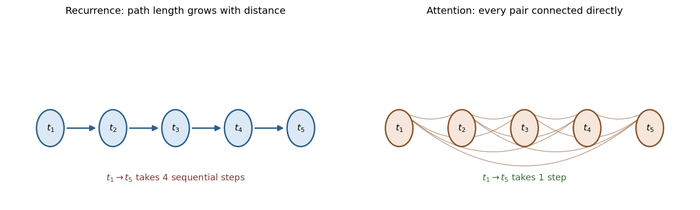
The Problem Attention Solves
RNNs: Sequential Bottleneck - Process tokens one at a time; hidden state updated at each step - Information from earlier tokens degrades over many steps (long-range decay) - No parallelism: step \(t\) waits for step \(t-1\) (inefficient on modern hardware)
Attention: Direct & Parallel - Every token sees all others in one operation - Any dependency uses a single step - Enables full parallel computation with matrix multiplications
The Core Idea
Attention is a learned, content-based weighted average
- Each token emits a query: a description of the information it is looking for
- Each token emits a key: a description of the information it can offer
- Each token emits a value: the information it actually contributes
- A token’s output is the average of all values, weighted by how well its query matches each key
Why this is powerful
- The weights are computed from the content of the tokens themselves, not fixed in advance
- The word
satcan pull incatbecause their query and key happen to align, regardless of how far apart they sit - Nothing here is sequential, (sequence is encoded in the position embeddings) so the whole sentence is processed at once
Step 1: From Text to Vectors
The Corpus and the Vocabulary
Our entire training corpus is one sentence
the cat sat
Tokenization
- Splitting on whitespace gives three tokens, so the sequence length is \(n = 3\)
- Real systems use subword tokenization such as byte pair encoding, which splits rare words into pieces; that detail does not change anything below
The vocabulary and its integer index
| index | token |
|---|---|
| 0 | the |
| 1 | cat |
| 2 | sat |
- Vocabulary size \(|V| = 3\)
- At this point a token is just an integer with no meaning attached to it
Token Embeddings: A Lookup Table
Definition
- An embedding is a dense vector of real numbers that represents a token
- The embedding matrix \(W_E \in \mathbb{R}^{|V| \times d_{\text{model}}}\) has one row per vocabulary entry
- Embedding a token is literally a row lookup:
\[e_t = W_E[\text{id}(w_t), :]\]
- In a real model \(W_E\) is learned by gradient descent. Here we pick it by hand
Our lookup table, with \(d_{\text{model}} = 4\)
| token | embedding \(e\) |
|---|---|
the |
\((1,\; 0,\; 0,\; 0)\) |
cat |
\((0,\; 1,\; 0,\; 0)\) |
sat |
\((0,\; 0,\; 1,\; 0)\) |
- Coordinates 1 to 3 act as an identity slot, one per word
- Coordinate 4 is deliberately left empty. Position will live there
Positional Encoding: Putting Order Back In
Why it is needed
- Attention computes a weighted average over positions
- An average does not care about order, so
cat sat theandthe cat satwould look identical to it - The fix is to add order information into the vectors themselves before attention ever sees them
Our toy positional lookup table
- One learned row per position \(t\):
\[p_t = (0,\; 0,\; 0,\; t)\]
| position \(t\) | \(p_t\) |
|---|---|
| 1 | \((0,0,0,1)\) |
| 2 | \((0,0,0,2)\) |
| 3 | \((0,0,0,3)\) |
How the original paper did it
- The 2017 paper used fixed sinusoids of many different frequencies, \(\sin(t / 10000^{2i/d})\) and \(\cos(t / 10000^{2i/d})\), so that relative offsets are easy to express
- Most modern models use learned position embeddings or rotary encodings instead. The mechanism is the same: add a position-dependent vector
Step 3: The Input Matrix \(X\)
Embedding and position are added, not concatenated
\[x_t = e_t + p_t\]
Working it out
- \(x_1 = (1,0,0,0) + (0,0,0,1) = (1,\;0,\;0,\;1)\)
- \(x_2 = (0,1,0,0) + (0,0,0,2) = (0,\;1,\;0,\;2)\)
- \(x_3 = (0,0,1,0) + (0,0,0,3) = (0,\;0,\;1,\;3)\)
Stack the rows into one matrix
\[X = \begin{bmatrix} 1 & 0 & 0 & 1 \\ 0 & 1 & 0 & 2 \\ 0 & 0 & 1 & 3 \end{bmatrix} \in \mathbb{R}^{3 \times 4}\]
- Row \(t\) is the vector for position \(t\); this row-per-token convention holds for every matrix in this deck
- Shape is \(n \times d_{\text{model}}\), and it stays \(n \times d_{\text{model}}\) all the way through the encoder
Step 2: Self-Attention
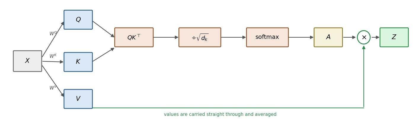
Queries, Keys, and Values
Each input generates three vectors:
- Query: what we’re searching for
- Key: labels for each entry
- Value: content to retrieve
Unlike databases (hard lookup), attention returns a weighted average of all values:
- Weights reflect how closely each key matches the query (via dot product)
All are computed as linear projections of input \(X\):
\[ Q = X W^Q, \quad K = X W^K, \quad V = X W^V \]
\(W^Q, W^K \in \mathbb{R}^{d_{\text{model}} \times d_k}\), \(W^V \in \mathbb{R}^{d_{\text{model}} \times d_v}\) (all learned)
Step 4: Our Projection Matrices
We use \(d_k = d_v = 2\), so each matrix is \(4 \times 2\). Rows correspond to input coordinates: the slot, cat slot, sat slot, position slot.
Query matrix. Read it as: verbs go looking for nouns, nouns go looking for verbs.
\[W^Q = \begin{bmatrix} 0 & 0 \\ 0 & 2 \\ 2 & 0 \\ 0 & 0 \end{bmatrix}\]
Key matrix. Read it as: coordinate 1 advertises “I am a noun”, coordinate 2 advertises “I am a verb”.
\[W^K = \begin{bmatrix} 0 & 0 \\ 1 & 0 \\ 0 & 1 \\ 0 & 0 \end{bmatrix}\]
Value matrix. Coordinate 1 carries a word identity code, coordinate 2 carries the position.
\[W^V = \begin{bmatrix} 1 & 0 \\ 4 & 0 \\ 2 & 0 \\ 0 & 1 \end{bmatrix}\]
- A real model discovers matrices like these from data. We are short-circuiting the training so the pattern is visible
Step 5: Computing \(Q\), \(K\), and \(V\)
Each is one matrix product. For example, row 3 of \(Q\):
\[q_3 = x_3 W^Q = (0,0,1,3) \, W^Q = 1 \cdot (2,0) + 3 \cdot (0,0) = (2,\, 0)\]
All three results
\[Q = \begin{bmatrix} 0 & 0 \\ 0 & 2 \\ 2 & 0 \end{bmatrix}, \quad K = \begin{bmatrix} 0 & 0 \\ 1 & 0 \\ 0 & 1 \end{bmatrix}, \quad V = \begin{bmatrix} 1 & 1 \\ 4 & 2 \\ 2 & 3 \end{bmatrix}\]
Reading the rows
- \(q_1 = (0,0)\):
theis a function word and asks for nothing in particular - \(q_2 = (0,2)\):
catis looking for a verb - \(q_3 = (2,0)\):
satis looking for a noun - \(k_2 = (1,0)\):
catadvertises itself as a noun - \(k_3 = (0,1)\):
satadvertises itself as a verb - \(v_2 = (4,2)\): the content
catwill hand over, tagged with its position \(2\)
Step 6: Raw Compatibility Scores
Score every query against every key with a dot product
\[\text{score}(i,j) = q_i \cdot k_j\]
- A large positive score means position \(i\) finds position \(j\) relevant
- Doing this for all pairs at once is a single matrix product, \(Q K^{\top}\), of shape \(n \times n\)
Our scores
\[Q K^{\top} = \begin{bmatrix} 0 & 0 & 0 \\ 0 & 0 & 2 \\ 0 & 2 & 0 \end{bmatrix}\]
Checking one entry by hand
- Row 3, column 2 asks how much
satcares aboutcat - \(q_3 \cdot k_2 = (2,0) \cdot (1,0) = 2 \cdot 1 + 0 \cdot 0 = 2\)
- Compare row 3, column 3: \(q_3 \cdot k_3 = (2,0) \cdot (0,1) = 0\), so
satfinds itself uninformative - Row 1 is all zeros because \(q_1 = (0,0)\), so
thehas no preference at all
Step 7: Why Divide by \(\sqrt{d_k}\)
The problem
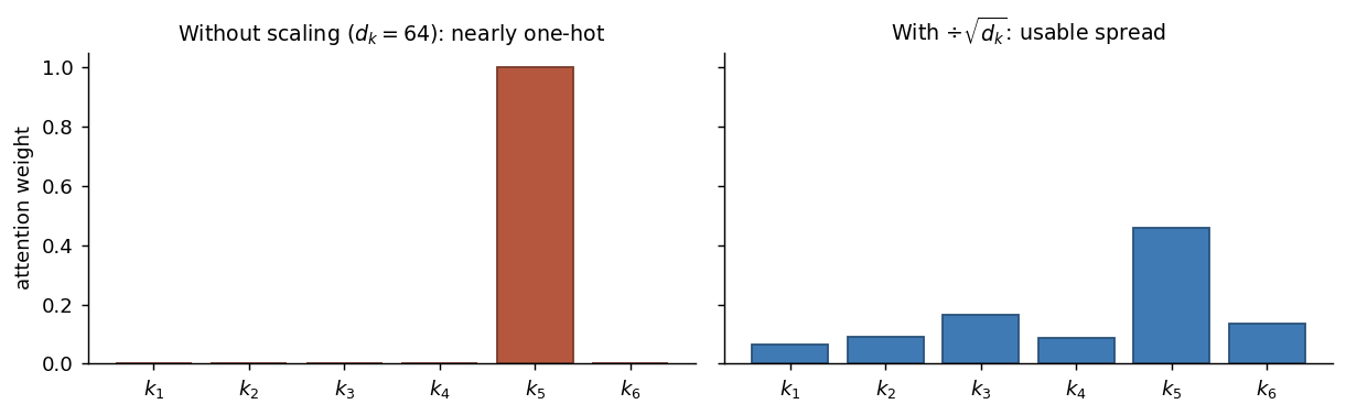
- A dot product of two \(d_k\)-dimensional vectors is a sum of \(d_k\) terms
- If the entries are roughly independent with variance \(1\), the dot product has variance about \(d_k\), so its typical size grows like \(\sqrt{d_k}\)
- With \(d_k = 64\) or \(512\), raw scores can easily reach the tens or hundreds
Why that hurts
- The softmax of very large scores is nearly one-hot: one weight close to \(1\), the rest close to \(0\)
- In that regime the gradient of the softmax is close to zero, so learning stalls before it starts
The fix: scaled dot-product attention
\[\text{score}(i,j) = \frac{q_i \cdot k_j}{\sqrt{d_k}}\]
- With \(d_k = 2\) our scaled score matrix is
\[S = \frac{1}{\sqrt{2}} \begin{bmatrix} 0 & 0 & 0 \\ 0 & 0 & 2 \\ 0 & 2 & 0 \end{bmatrix} = \begin{bmatrix} 0 & 0 & 0 \\ 0 & 0 & 1.414 \\ 0 & 1.414 & 0 \end{bmatrix}\]
Step 8: Softmax Turns Scores into Weights
Definition
- The softmax converts a row of real numbers into positive numbers that sum to \(1\)
\[\alpha_{ij} = \frac{\exp(S_{ij})}{\sum_{j'=1}^{n} \exp(S_{ij'})}\]
- It is applied row by row, so each query gets its own probability distribution over positions
Row 3 worked out, the query from sat
- Scaled scores: \((0,\; 1.414,\; 0)\)
- Exponentiate: \(e^{0} = 1\), \(e^{1.414} = 4.113\), \(e^{0} = 1\)
- Sum: \(1 + 4.113 + 1 = 6.113\)
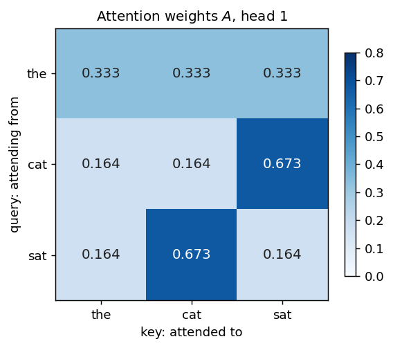
- Divide: \(\alpha_3 = (0.164,\; 0.673,\; 0.164)\)
The full attention matrix
\[A = \begin{bmatrix} 0.333 & 0.333 & 0.333 \\ 0.164 & 0.164 & 0.673 \\ 0.164 & 0.673 & 0.164 \end{bmatrix}\]
- Every row sums to \(1\)
- Row 1 is uniform, which is exactly what a zero query should give
Step 9: The Weighted Sum of Values
Each output row is a convex combination of the value rows
\[z_i = \sum_{j=1}^{n} \alpha_{ij} \, v_j\]
- Equivalently, all rows at once: \(Z = A V\)
Row 3 worked out, the output for sat
- Weights \(\alpha_3 = (0.164,\, 0.673,\, 0.164)\) and values \(v_1 = (1,1)\), \(v_2 = (4,2)\), \(v_3 = (2,3)\)
- First coordinate: \(0.164(1) + 0.673(4) + 0.164(2) = 0.164 + 2.691 + 0.327 = 3.182\)
- Second coordinate: \(0.164(1) + 0.673(2) + 0.164(3) = 0.164 + 1.346 + 0.491 = 2.000\)
- So \(z_3 = (3.182,\; 2.000)\)
All three outputs of head 1
\[Z^{(1)} = \begin{bmatrix} 2.333 & 2.000 \\ 2.164 & 2.509 \\ 3.182 & 2.000 \end{bmatrix}\]
The Result
cat’s value is \(v_2 = (4,2)\) (largest code in the vocab).- Before attention: position 3 has no info about
cat. - After attention: \(z_3 = (3.182, 2.000)\), close to \(v_2\), since \(67\%\) of the weight went to
cat. - The verb’s output now encodes its subject—achieved in a single attention step (no recurrence).
Position 1 Observation - the yields a zero query → uniform attention → output is the mean of all values. - Uninformative tokens summarize the sentence—seen in real models.
Caveat - Here, \(W^Q\) and \(W^K\) ignore position info; \(W^V\) can still encode position, and other heads may use it.
The Whole Mechanism in One Equation
\[\text{Attention}(Q, K, V) = \text{softmax}\!\left( \frac{Q K^{\top}}{\sqrt{d_k}} \right) V\]
Shape bookkeeping, with \(n\) tokens
- \(Q\) is \(n \times d_k\), \(K\) is \(n \times d_k\), \(V\) is \(n \times d_v\)
- \(Q K^{\top}\) is \(n \times n\), one score per ordered pair of tokens
- softmax leaves the shape alone and normalizes each row
- Multiplying by \(V\) gives \(n \times d_v\), one output vector per token
Three properties worth remembering
- Permutation equivariance. Without positional encoding, shuffling the input shuffles the output identically. Order comes only from \(p_t\)
- Parallelism. Two matrix products and a softmax, no loop over time
- Quadratic cost. The \(n \times n\) score matrix is the price of connecting everything to everything
Step 3: Multi-Head Attention
Why Not Just One Attention Head?
One attention head only captures a single type of relationship.
- Ex: “verbs attend to nouns”
- But sentences involve many relations:
- subject–verb agreement
- pronoun reference
- local context (adjacent tokens)
- topical links across sentence
Solution: apply multiple attention heads in parallel.
Model width split into \(h\) heads, each with \(d_k = d_v = d_\text{model}/h\)
Each head has its own \(W^Q_i\), \(W^K_i\), \(W^V_i\): learns different patterns
Outputs from all heads are concatenated, then mixed via \(W^O\)
\[\text{MultiHead}(X) = \text{Concat}(\text{head}_1, \dots, \text{head}_h) W^O\]
\[\text{head}_i = \text{Attention}(X W^Q_i, X W^K_i, X W^V_i)\]
- Total compute stays similar since each head is narrower by \(h\)
Step 10: Concatenate and Project
Our second head is a simple averaging head
- Head 2 uses \(W^Q_2 = W^K_2 = 0\), so all its scores are zero and its attention is uniform
- Its values are \(v_1 = (1,0)\), \(v_2 = (0,1)\), \(v_3 = (1,1)\), so every position receives the same average
\[Z^{(2)} = \begin{bmatrix} 0.667 & 0.667 \\ 0.667 & 0.667 \\ 0.667 & 0.667 \end{bmatrix}\]
- This is a “sentence gist” head: it hands every token a summary of the whole sequence
Concatenate the two heads, \(2 + 2 = 4 = d_{\text{model}}\)
\[U = \left[ Z^{(1)} \;\middle|\; Z^{(2)} \right] = \begin{bmatrix} 2.333 & 2.000 & 0.667 & 0.667 \\ 2.164 & 2.509 & 0.667 & 0.667 \\ 3.182 & 2.000 & 0.667 & 0.667 \end{bmatrix}\]
Project back with \(W^O \in \mathbb{R}^{4 \times 4}\)
- We take \(W^O = I\) for readability, so \(\text{MultiHead}(X) = U\)
- In a real model \(W^O\) lets the layer blend information across heads rather than keeping them in separate lanes
# Step 4: The Rest of the Encoder Block
Residual Connections & Layer Normalization
- Residual Connection:
- Output adds sublayer result to input, not replaces it.
- \[\text{output} = \text{LayerNorm}(x + \text{Sublayer}(x))\]
- Sublayer only learns a correction; direct gradients enable deep training.
- Layer Normalization:
- Applied row-wise to token vectors in matrix \(U \in \mathbb{R}^{\text{sequence length} \times d_\text{model}}\).
- For token vector \(a\) (a row of \(U\)): \[
\text{LN}(a) = \gamma \odot \frac{a - \mu}{\sqrt{\sigma^2 + \epsilon}} + \beta
\]
- \(\mu\): mean of \(a\); \(\sigma^2\): variance; \(d = d_\text{model}\)
- \(\gamma, \beta\): learned per-feature parameters; \(\epsilon\): small constant.
- Standardizes each token’s features (columns), not across tokens or batch.
- Keeps activations stable as residuals are added.
- Row-wise normalization is flexible for varying sequence length inputs.
Step 11: Add and Norm, Worked at Position 3
Add the residual
- \(x_3 = (0,\; 0,\; 1,\; 3)\) and \(\text{MultiHead}(X)_3 = (3.182,\; 2.000,\; 0.667,\; 0.667)\)
- Sum: \(r_3 = (3.182,\; 2.000,\; 1.667,\; 3.667)\)
Normalize, taking \(\gamma = 1\) and \(\beta = 0\)
- Mean: \(\mu = \dfrac{3.182 + 2.000 + 1.667 + 3.667}{4} = 2.629\)
- Variance: \(\sigma^2 = 0.676\), so \(\sigma = 0.822\)
- Subtract and divide, coordinate by coordinate:
- \((3.182 - 2.629)/0.822 = 0.673\)
- \((2.000 - 2.629)/0.822 = -0.765\)
- \((1.667 - 2.629)/0.822 = -1.170\)
- \((3.667 - 2.629)/0.822 = 1.262\)
\[h_3 = (0.673,\; -0.765,\; -1.170,\; 1.262)\]
- Sanity check: these four numbers have mean \(0\) and standard deviation \(1\), which is the whole point
The Position-Wise Feed-Forward Network
What it is
- A two-layer multilayer perceptron applied to each position separately, with shared weights
\[\text{FFN}(h) = \text{ReLU}(h W_1 + b_1)\, W_2 + b_2\]
- \(W_1 \in \mathbb{R}^{d_{\text{model}} \times d_{ff}}\) expands, \(W_2 \in \mathbb{R}^{d_{ff} \times d_{\text{model}}}\) contracts
- Typically \(d_{ff} = 4 \, d_{\text{model}}\), so \(512 \rightarrow 2048 \rightarrow 512\) in the original paper
- ReLU is the rectifier \(\text{ReLU}(u) = \max(u, 0)\), which zeroes out negatives
Why it is there
- Attention is a weighted average of values, which is a linear operation once the weights are fixed
- Stacking averages without a nonlinearity in between would collapse toward a single linear map
- The feed-forward network supplies the per-token nonlinear processing, while attention supplies the mixing across tokens
- A useful slogan: attention moves information between positions, the feed-forward network transforms it in place
Step 12: The Feed-Forward Network, Worked
Our toy weights, with \(d_{ff} = 8\) and \(b_1 = b_2 = 0\)
- \(W_1 = [\, I_4 \;|\; -I_4 \,]\), which is \(4 \times 8\): the first four hidden units see \(h\), the last four see \(-h\)
- \(W_2 = \begin{bmatrix} I_4 \\ -0.5\, I_4 \end{bmatrix}\), which is \(8 \times 4\)
- Net effect, coordinate by coordinate: \(\text{ReLU}(u) - 0.5\,\text{ReLU}(-u)\), a leaky rectifier
- Real networks use dense learned matrices; this structured choice just keeps the numbers checkable
Applied to \(h_3 = (0.673,\; -0.765,\; -1.170,\; 1.262)\)
- Hidden layer before ReLU: \((0.673, -0.765, -1.170, 1.262,\; -0.673, 0.765, 1.170, -1.262)\)
- After ReLU: \((0.673,\; 0,\; 0,\; 1.262,\; 0,\; 0.765,\; 1.170,\; 0)\)
- Contract with \(W_2\):
- coordinate 1: \(0.673 - 0.5(0) = 0.673\)
- coordinate 2: \(0 - 0.5(0.765) = -0.382\)
- coordinate 3: \(0 - 0.5(1.170) = -0.585\)
- coordinate 4: \(1.262 - 0.5(0) = 1.262\)
\[\text{FFN}(h_3) = (0.673,\; -0.382,\; -0.585,\; 1.262)\]
Step 13: Second Add and Norm
Add the residual again
- \(h_3 + \text{FFN}(h_3) = (1.346,\; -1.147,\; -1.755,\; 2.524)\)
Normalize again
- Mean \(\mu = 0.242\), standard deviation \(\sigma = 1.757\)
- Result:
\[\text{EncoderBlock}(X)_3 = (0.628,\; -0.791,\; -1.137,\; 1.299)\]
All three positions
\[\text{EncoderBlock}(X) = \begin{bmatrix} 1.556 & -0.012 & -1.213 & -0.331 \\ -0.193 & 1.304 & -1.463 & 0.351 \\ 0.628 & -0.791 & -1.137 & 1.299 \end{bmatrix}\]
The key structural fact
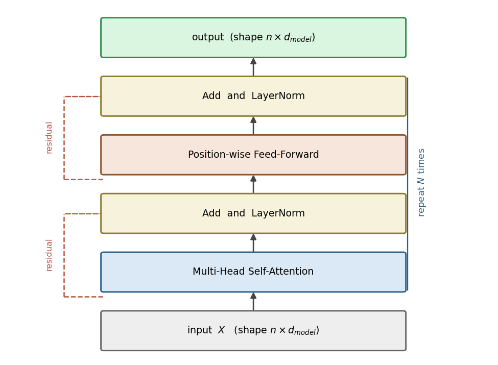
- Input was \(3 \times 4\) and output is \(3 \times 4\)
- Shape is preserved, which is exactly why blocks can be stacked without any glue between them
Stacking the Block
Depth comes from repetition, not variety
- The encoder is the same block repeated \(N\) times, each copy with its own weights
- The original paper used \(N = 6\) with \(d_{\text{model}} = 512\) and \(h = 8\) heads
- Modern large models use the same recipe with \(N\) in the dozens and widths in the thousands
What extra depth buys
- One layer lets a token gather from tokens
- Two layers let a token gather from tokens that have themselves already gathered, which builds indirect, multi-hop relationships
- Empirically, early layers tend to capture local and syntactic structure while later layers capture more abstract, task-relevant structure
The residual stream view
- Each token has a running \(d_{\text{model}}\)-dimensional vector
- Every sublayer reads from it and adds a correction back into it
- Nothing is ever overwritten wholesale, which is why information can survive dozens of layers
What Attention Costs
Compute and memory
- The score matrix \(QK^{\top}\) has \(n^2\) entries, so both time and memory scale as \(O(n^2 d)\)
- Doubling the context length quadruples the attention cost
- A recurrent network is \(O(n d^2)\), linear in \(n\), but strictly sequential
The tradeoff in one line
| attention | recurrence | |
|---|---|---|
| max path length | \(O(1)\) | \(O(n)\) |
| parallel over positions | yes | no |
| cost in \(n\) | quadratic | linear |
Why the tradeoff was worth it
- Sequence lengths are usually far smaller than model widths, so the quadratic term is affordable
- Full parallelism is what allowed training to scale to enormous datasets
- Long-context research is largely about restoring near-linear cost while keeping the direct paths
Encoder vs Decoder
Encoder (what we built) - Self-attention with no mask: every position attends to all others - Used for tasks where full input is available (e.g., classification, tagging) - Basis for encoder-only models (e.g., BERT)
Decoder (adds two features) - Causal masking: positions \(j > i\) set to \(-\infty\) before softmax, so no peeking at future tokens - Cross-attention: queries from decoder, keys/values from encoder output (enables source-target mapping in translation)
Summary - Decoder-only stacks with causal masking are standard for generative models - The core block—attention, feed-forward, residual, normalization—remains unchanged
Summary
The five moves of self-attention
- Project. \(Q = XW^Q\), \(K = XW^K\), \(V = XW^V\)
- Score. \(QK^{\top}\) compares every query to every key
- Scale. Divide by \(\sqrt{d_k}\) to keep the softmax out of its saturated regime
- Normalize. Row-wise softmax gives weights that sum to \(1\)
- Average. Multiply by \(V\) to blend the values
\[\text{Attention}(Q,K,V) = \text{softmax}\!\left(\frac{QK^{\top}}{\sqrt{d_k}}\right) V\]
The four things wrapped around it
- Positional encoding, because averaging is order blind
- Multiple heads, because one notion of relevance is not enough
- Residual connections and layer normalization, because depth needs stable gradients and stable scales
- A position-wise feed-forward network, because mixing alone is not enough without a nonlinearity
The single sentence to remember
- A transformer encoder repeatedly lets every token look at every other token, decide what is relevant from content, and update itself with a weighted summary of what it found