import networkx as nx
import matplotlib.pyplot as plt
#FUNCTION FOR NETWORK PLOTTING
# def draw_network(G):
# #CUSTOMIZE GRAPH A BIT
# pos= nx.circular_layout(G)
# nx.draw(G,
# with_labels=True,
# node_color='blue',
# node_size=1600,
# pos=pos,
# font_color='white',
# font_size=16,
# )
# plt.show()
def draw_network(G):
#COMPUTE DEGREE: --> "LIST" WITH NODE DEGREES
G_DEGREE=G.degree(); #print(G_DEGREE,G_DEGREE[5],type(G_DEGREE))
# #LABELS (DICT)
# labels={}
# for n,d in G_DEGREE: labels[n]=d #str(n)+"-"+str(d)
#SORT DEGREE AND STORE IN LIST
degree_sequence = sorted((d for n, d in G_DEGREE), reverse=True)
dmax = max(degree_sequence) #MAX DEGREE
#INITIALIZE MPL FIGURE+AX
fig = plt.figure("Degree of a random graph", figsize=(12, 12))
# Create a gridspec for adding subplots of different sizes
axgrid = fig.add_gridspec(5, 4)
#PLOT NETWORK IN UPPER GRID SPACES
ax0 = fig.add_subplot(axgrid[0:3, :])
# pos = nx.spring_layout(G)
# pos= nx.circular_layout(G)
nx.draw(G,
with_labels=True,
# labels=labels,
node_color='blue',
node_size=500,
font_color='white',
font_size=16,
pos=pos,ax=ax0
)
ax0.set_title("Network Graph: G")
#PLOT RANK (IMPORTANCE BASED ON DEGREE) VS DEGREE)
ax1 = fig.add_subplot(axgrid[3:, :2])
ax1.plot(degree_sequence, "b-", marker="o")
ax1.set_title("Degree Rank Plot")
ax1.set_ylabel("Degree")
ax1.set_xlabel("Rank")
#PLOT RANK HISTOGRAM
ax2 = fig.add_subplot(axgrid[3:, 2:])
ax2.bar(*np.unique(degree_sequence, return_counts=True))
ax2.set_title("Degree histogram")
ax2.set_xlabel("Degree")
ax2.set_ylabel("# of Nodes")
ax0.set_aspect('equal', 'box')
fig.tight_layout()
plt.show()
Core decomposition
Network structure review
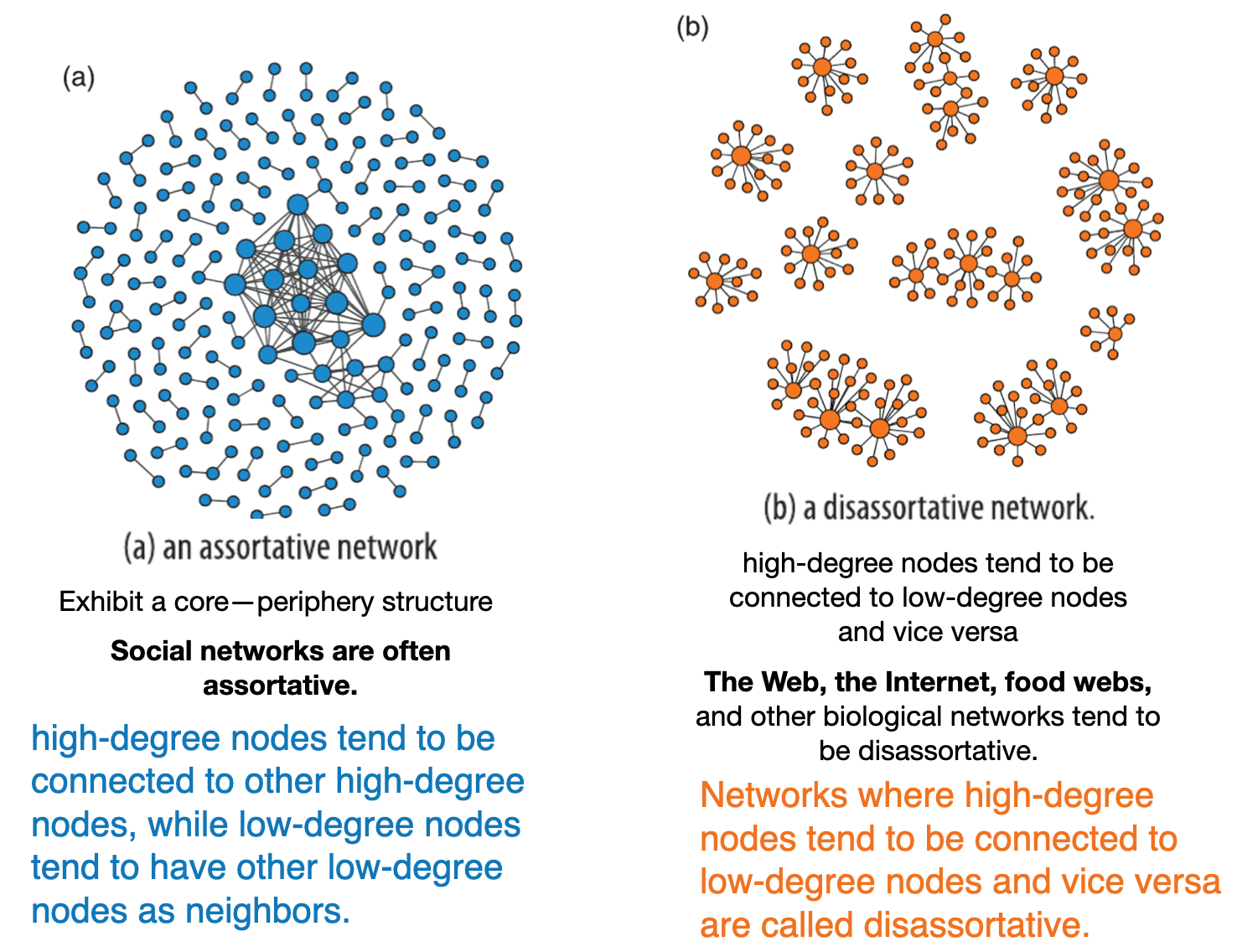
Recall: Assortative networks
Connected components
Connected Networks: A network where, for any node, there exists a path by which you can reach any other nodeYou can think of connected components as
islands, within the network- If a network is not connected, we say that it is disconnected;
Recall
density: i.e. a measure of graph’s connectivity.

- The following is often true, but not always.
higher the density —> more likely to be connectedlower the density —> less likely to be connected
Core: The core is a special name for the largest connected component
Code example
- Note:
nx.connected_components(G)returns a generator object (not ordered by size).- We can use the
nextfunction to get just the first item from the generator.
- We can use the
- The generator can be converted to a list using
list(nx.connected_components(G))- The length of this list is the number of connected components:
- Each component is provided as a set of node names:
import matplotlib.pyplot as plt
import numpy as np
import networkx as nx

def check_connectivity(G):
    print("----------------")
    print("Connected:",nx.is_connected(G))
    print("Density:",np.round(nx.density(G),3))
    print("Connected components:",list(nx.connected_components(G)))
    print("Number of connected components:",len(list(nx.connected_components(G))))

    # CC=nx.connected_components(G)
    # print(next(nx.connected_components(G)))
    nx.draw(G, with_labels=True, font_color="white")
    plt.show()

G = nx.complete_graph(10)
check_connectivity(G)

G = nx.star_graph(10)
check_connectivity(G)

G = nx.gnp_random_graph(10, 0.5, seed=10374196)
check_connectivity(G)

G = nx.gnp_random_graph(10, 0.2, seed=10374196)
check_connectivity(G)
----------------
Connected: True
Density: 1.0
Connected components: [{0, 1, 2, 3, 4, 5, 6, 7, 8, 9}]
Number of connected components: 1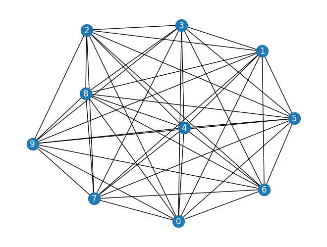
----------------
Connected: True
Density: 0.182
Connected components: [{0, 1, 2, 3, 4, 5, 6, 7, 8, 9, 10}]
Number of connected components: 1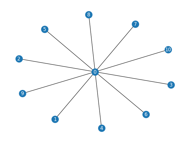
----------------
Connected: True
Density: 0.578
Connected components: [{0, 1, 2, 3, 4, 5, 6, 7, 8, 9}]
Number of connected components: 1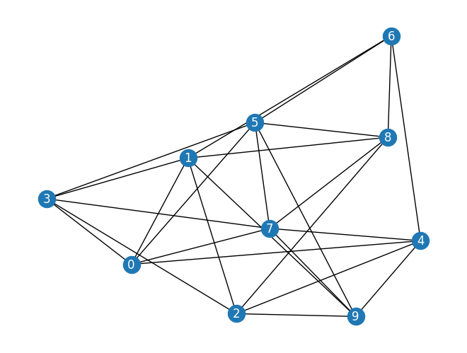
----------------
Connected: False
Density: 0.133
Connected components: [{0, 3}, {1, 2, 4, 6}, {8, 5}, {9, 7}]
Number of connected components: 4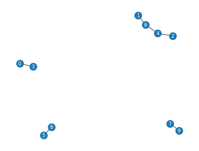
Core decomposition
Overview
- Core Decomposition Definition: A method to decompose a network into nested subgraphs, called k-cores, where each node is connected to at least k other nodes within the subgraph.
- K-Core: A maximal subgraph in which each vertex has at least degree k.
- Importance: Helps identify central and cohesive areas in a network.
- Algorithm: Typically involves iteratively removing nodes with degrees less than k until no such nodes remain.
- Applications: Used in social network analysis, biology, computer networks, and more to reveal the structure and hierarchies within networks.
Use-case: Visualizing the core
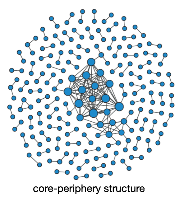
- When analyzing or visualizing a large network, it is often useful to focus on its denser portion (the core)
- Degree shells: The degree can be used to separate a network into distinct portions, called shells, based on their position in the core
- Low-degree: outer shells on the periphery.
- High-degree: core nodes
- As low degree nodes are removed, what remains is a denser and denser sub-network (i.e. the core)
- Core decomposition is particularly helpful in practice for filtering out peripheral nodes when visualizing large networks.
Core decomposition algorithm
Formally, the \(k\)-core decomposition algorithm starts by setting \(k=0\). Then it proceeds iteratively. Each iteration corresponds to a value of \(k\) and consists of a few simple steps:
- Recursively remove all nodes of degree \(k\), until there are no more left.
- The removed nodes make up the \(k\)-shell and the remaining nodes make up the \((k+\) 1)-core, because they all have degree \(k+1\) or larger.
- If there are no nodes left in the core, terminate; else, increment \(k\) for the next iteration.
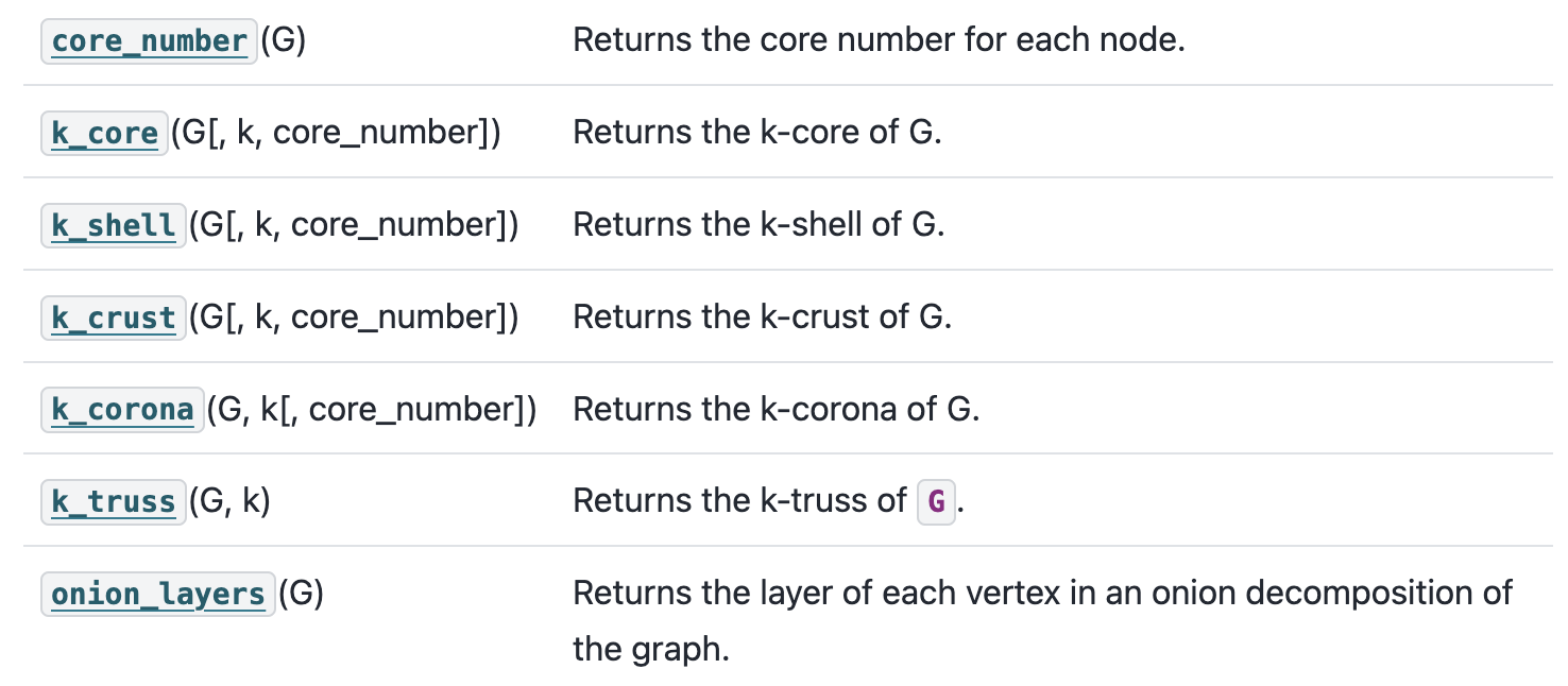
NetworkXhas functions for core decomposition:

Example: Political network
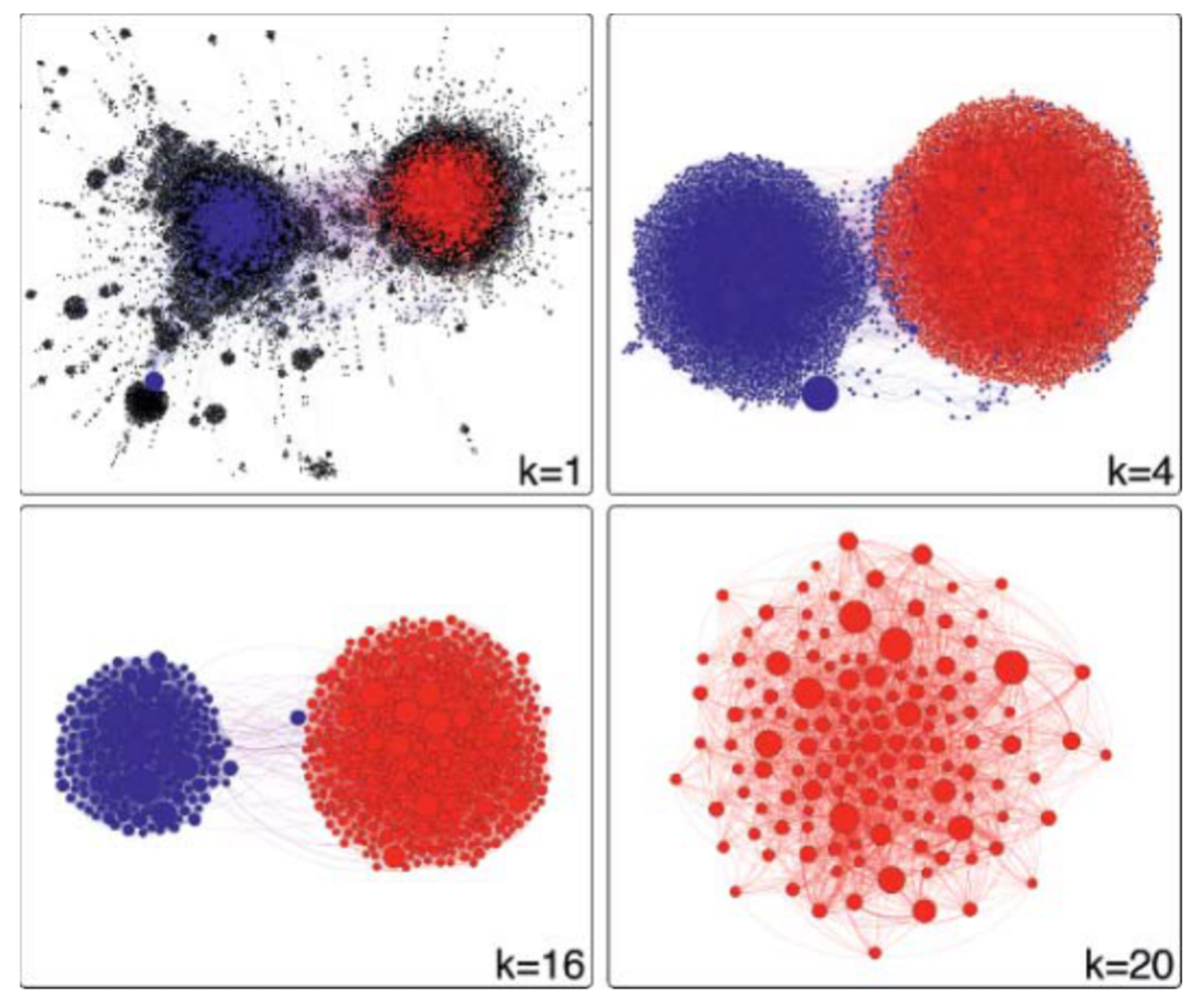
- Filtering by \(k\)-core decomposition. We start from the full Twitter political retweet network \((k=1)\).
- As we increase \(k\), peripheral nodes are removed and the remaining core becomes smaller and denser.
- The innermost core contains only red nodes, corresponding to conservative accounts; each has at least \(k=20\) neighbors.
Example: Physical network

Code example
Recall relevant functions
Utility function
Create and visualize network
Lets start with a random network with a density of 0.2 and add some singletons
N=20
G = nx.gnp_random_graph(N, 0.2, seed=10374196)
G.add_nodes_from([N+1,N+2,N+3])
pos= nx.circular_layout(G) # define globally
draw_network(G )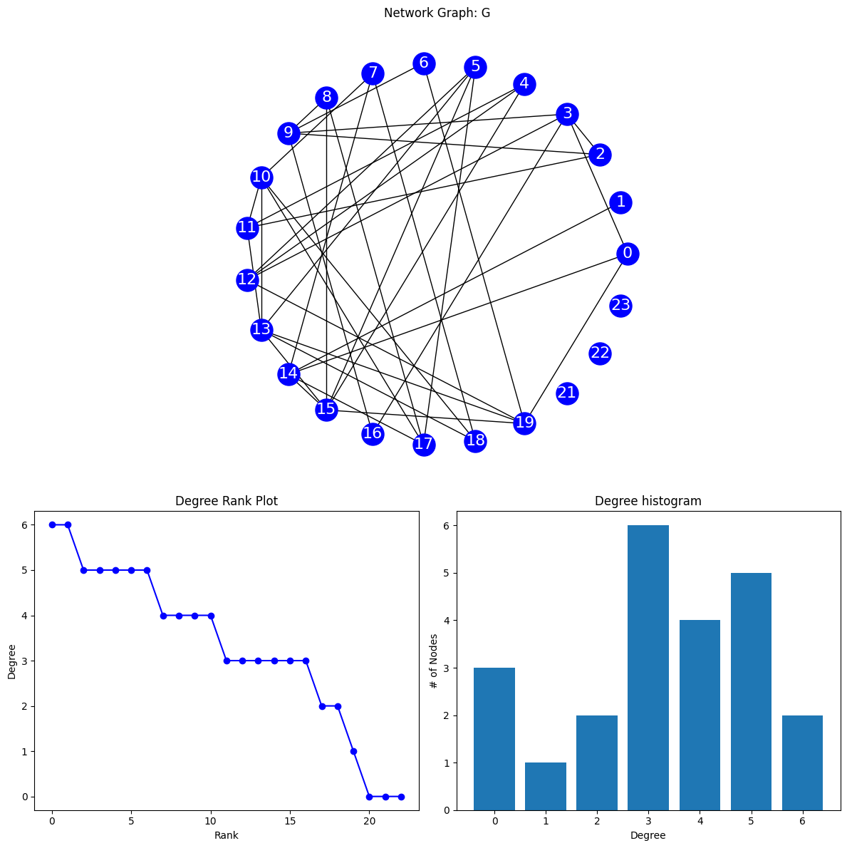
Core-Shell example: K=0
Gk=nx.k_core(G,0)
print(Gk)
draw_network(Gk)
Graph with 23 nodes and 38 edges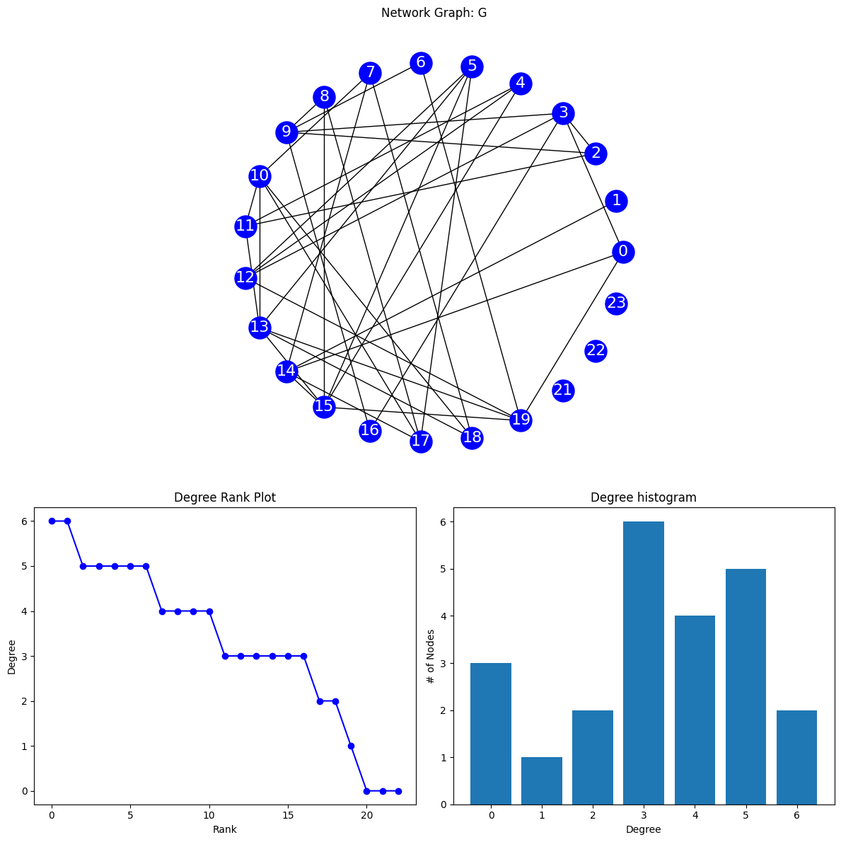
Gk=nx.k_shell(G,0)
print(Gk)
draw_network(Gk)
Graph with 3 nodes and 0 edges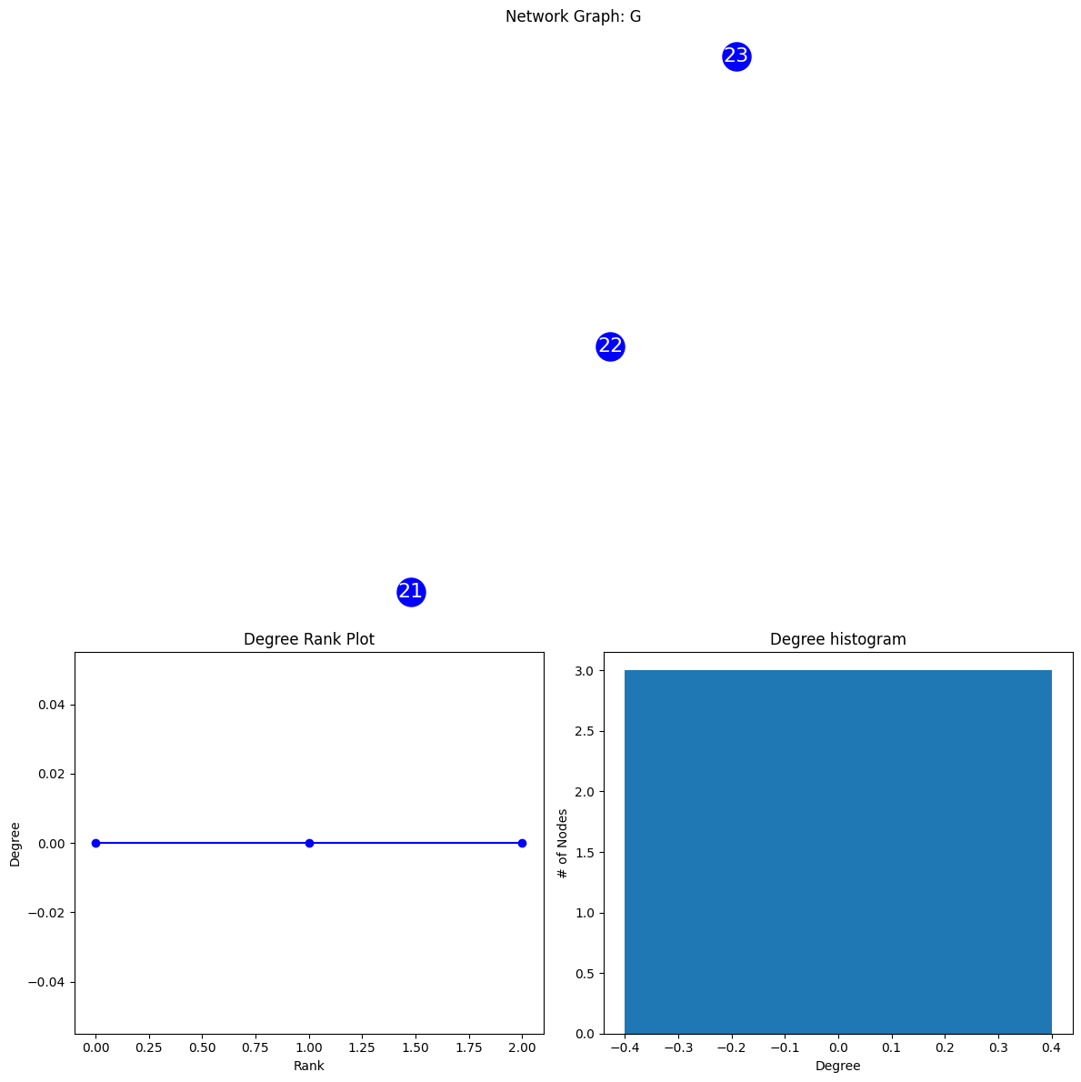
print(nx.core_number(G))
print(max(nx.core_number(G).values()))
{0: 3, 1: 1, 2: 3, 3: 3, 4: 3, 5: 3, 6: 2, 7: 3, 8: 3, 9: 3, 10: 3, 11: 3, 12: 3, 13: 3, 14: 3, 15: 3, 16: 2, 17: 3, 18: 3, 19: 3, 21: 0, 22: 0, 23: 0}
3Core-Shell example: K=1
Gk=nx.k_core(G,1)
print(Gk)
draw_network(Gk)
Graph with 20 nodes and 38 edges
Gk=nx.k_shell(G,1)
print(Gk)
draw_network(Gk)
Graph with 1 nodes and 0 edges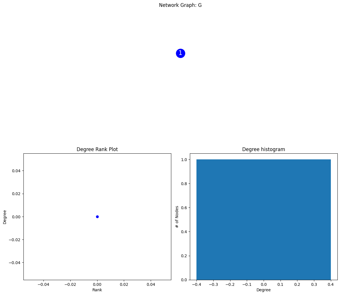
Compare to GCC
Notice how this is the same as K=1 (since removing the singletons leaves the GCC in this case)
def isolate_GCC(G):
    # get list of CC and return the first one in sorted list, i.e the larges one
    comps = sorted(nx.connected_components(G),key=len, reverse=True)
    nodes_in_giant_comp = comps[0]
    # return subgraph
    return nx.subgraph(G, nodes_in_giant_comp)

GCC=isolate_GCC(G)
draw_network(GCC)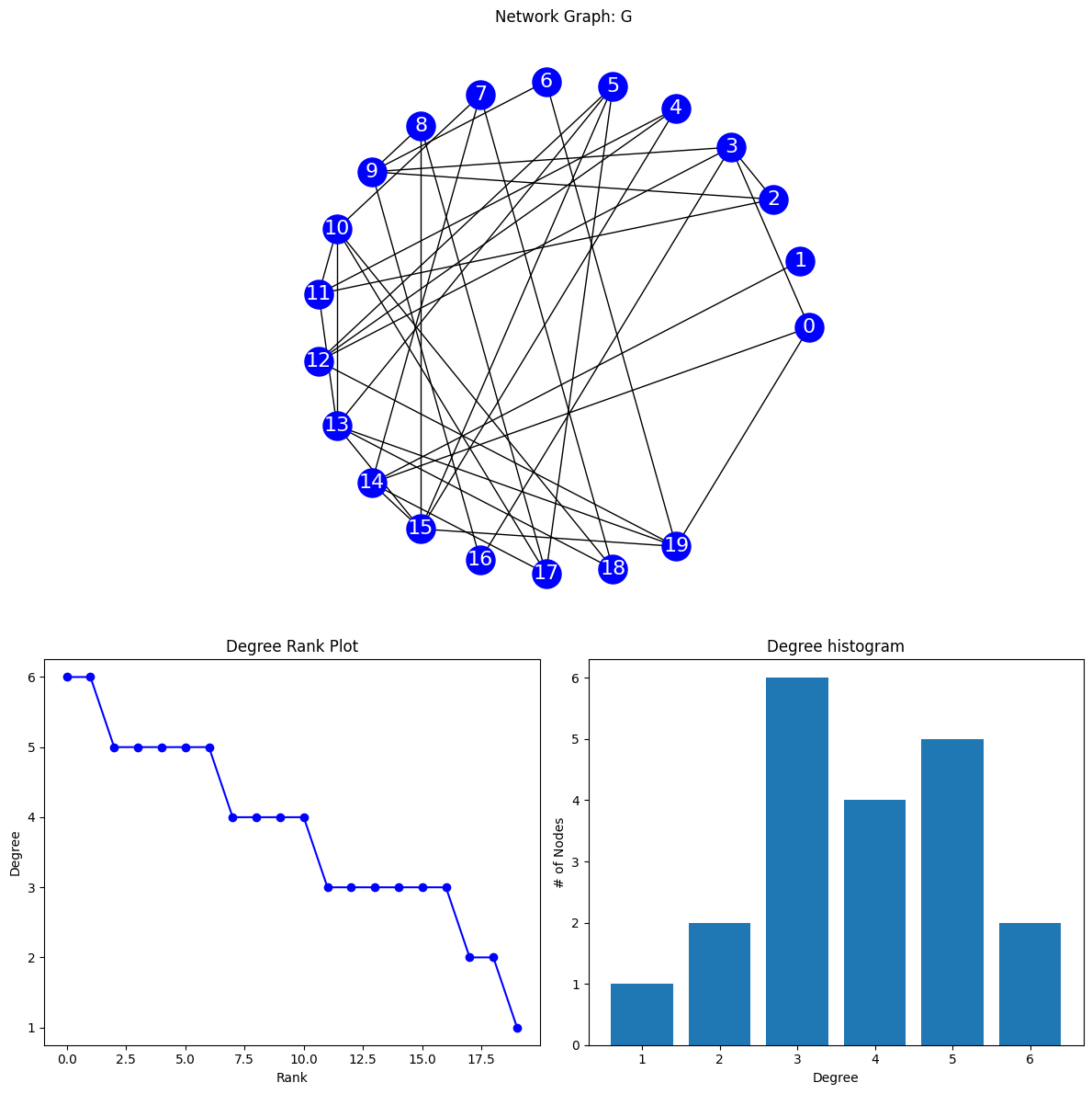
Core example: K=2
Gk=nx.k_core(G,2)
print(Gk)
draw_network(Gk)
Graph with 19 nodes and 37 edges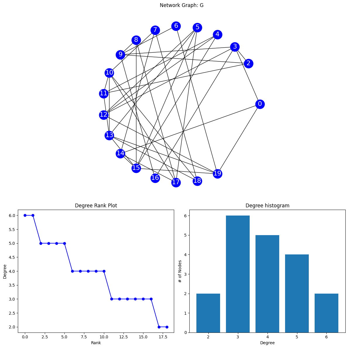
Gk=nx.k_shell(G,2)
print(Gk)
draw_network(Gk)
Graph with 2 nodes and 0 edges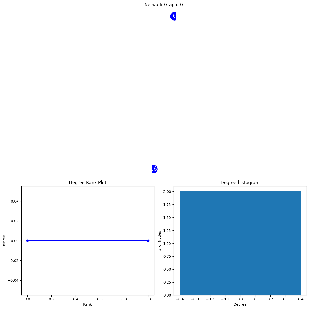
Crust of K=2 shell
The crust in core-shell decomposition refers to the subset of nodes in a network that belong to the outermost layers or lower-order cores.
- Nodes with the fewest connections
- Found in the outer layers of the network
- Less central and less influential
- Compared to nodes in higher-order cores
- Provides insight into the peripheral structure of the network
- Important for understanding network disintegration and interactions of peripheral nodes
crust=nx.k_shell(G,3)
print(crust)
draw_network(crust)
Graph with 17 nodes and 33 edges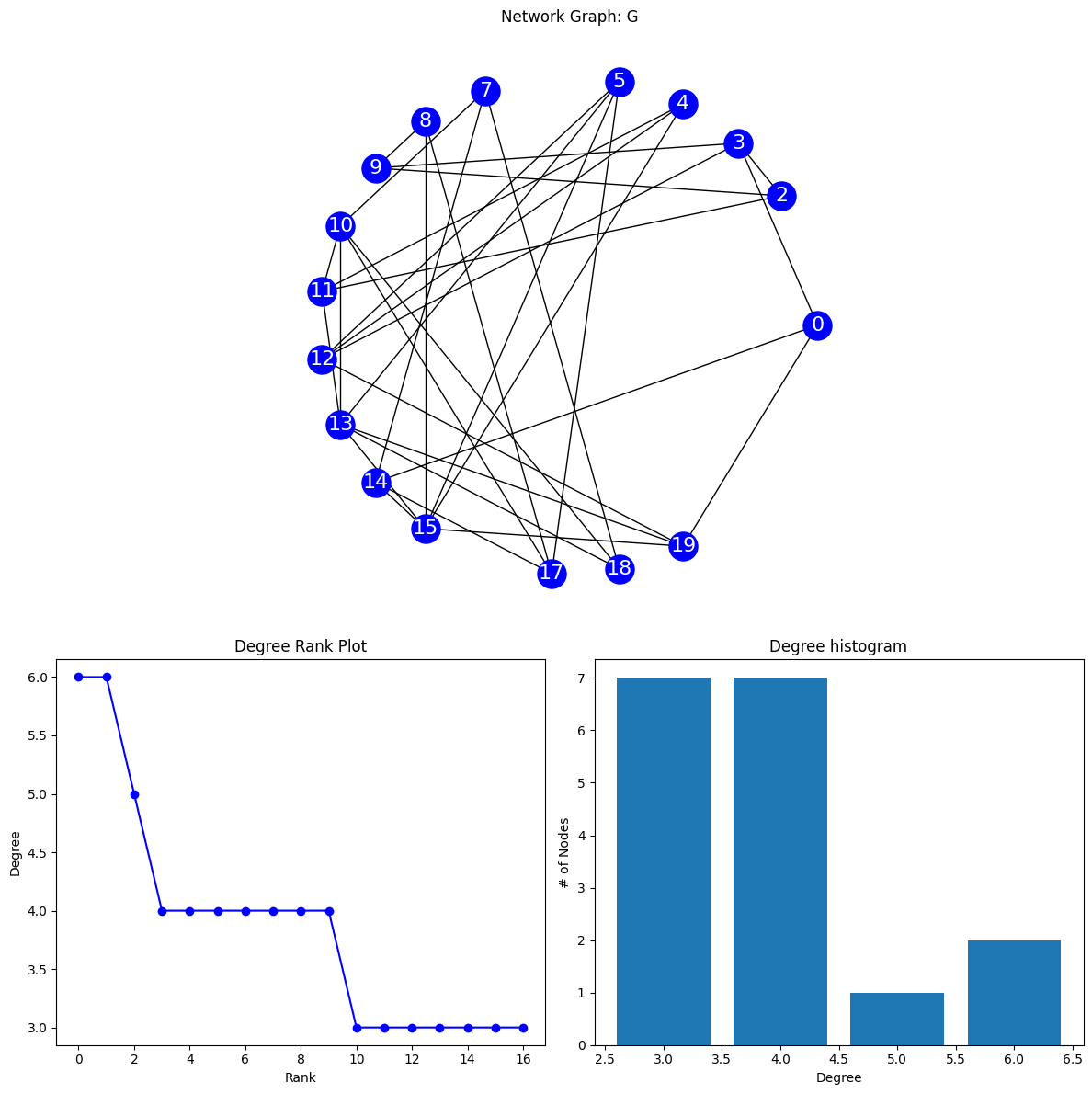
Shell example: K=3
Gk=nx.k_core(G,3)
print(Gk)
draw_network(Gk)
Graph with 17 nodes and 33 edges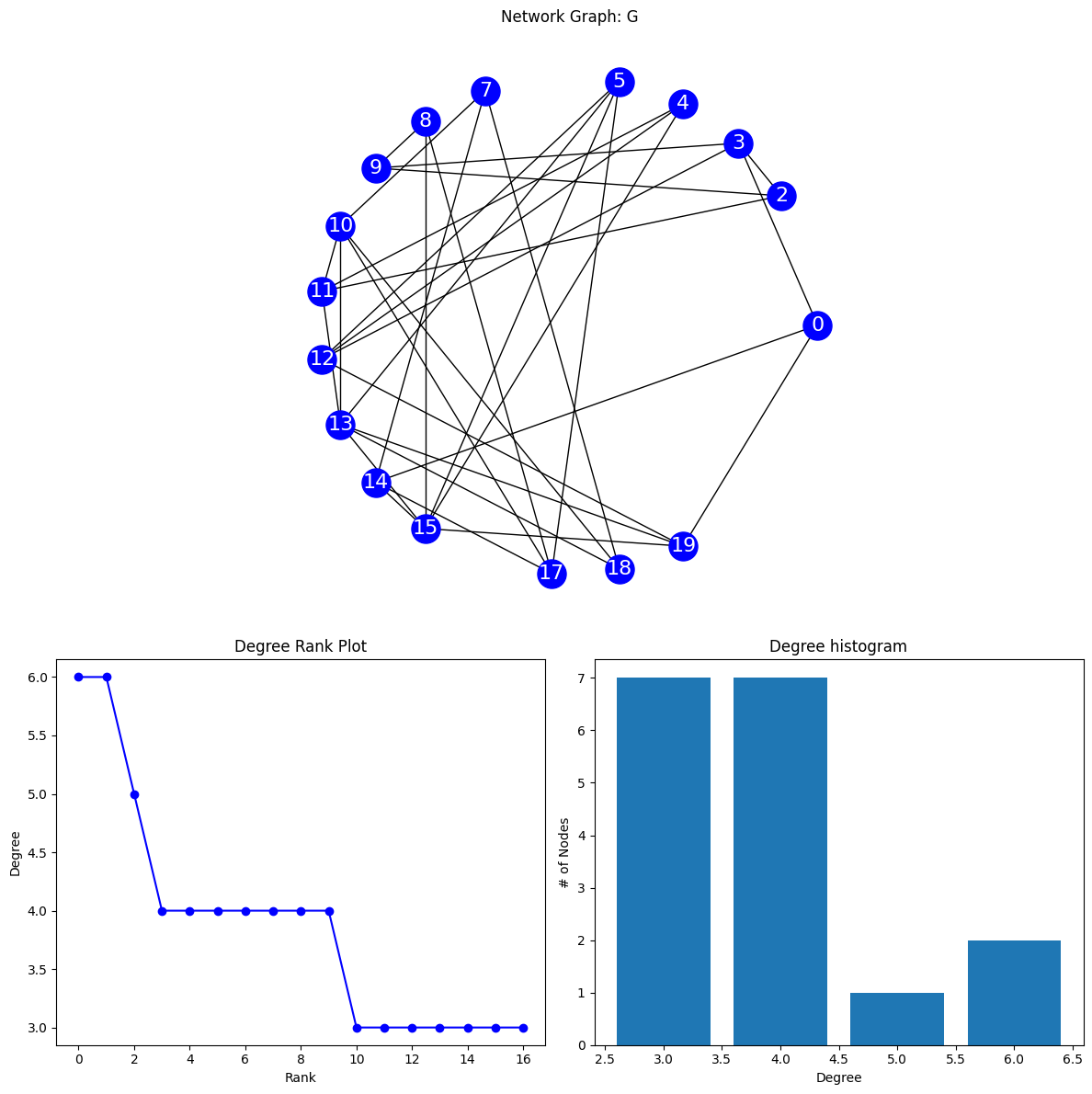
Gk=nx.k_shell(G,3)
print(Gk)
draw_network(Gk)
Graph with 17 nodes and 33 edges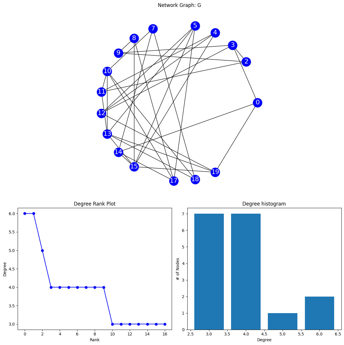
Coding from scratch
- Let’s explore why the algorithm stops at k=3.
- From the plots below, we can see that after k=3, removing nodes with 4 neighbors results in a graph where the degree of some remaining nodes is decreased by the removal.
- This is why the code terminates when it does.
- Removal condition appears to be that degree of nodes in remaining core is the same as the original network
# original network
draw_network(G)
print(nx.degree(G))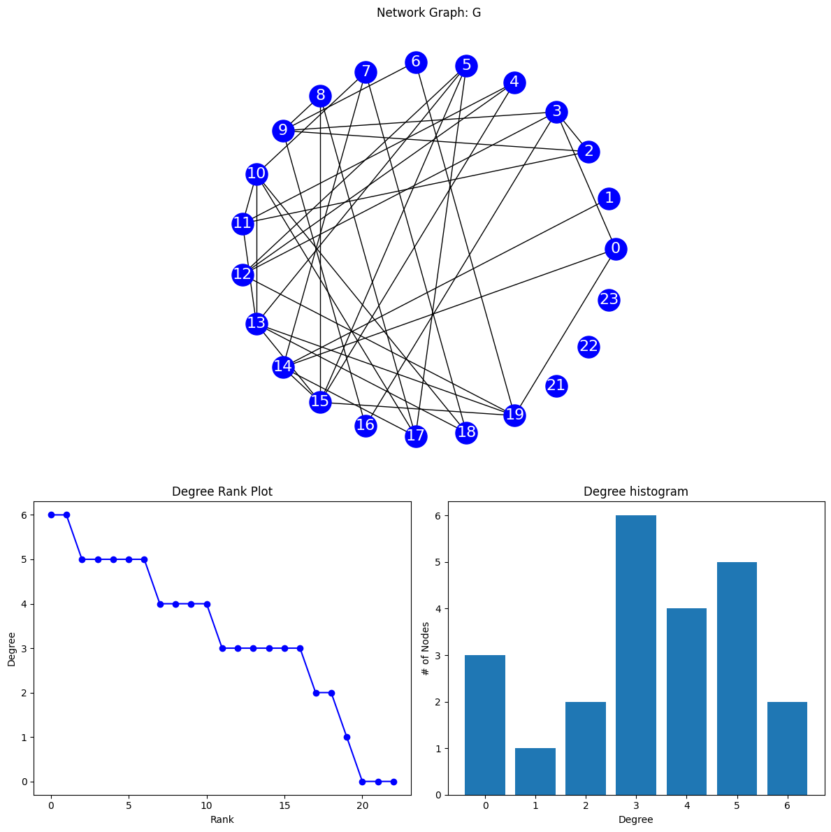
[(0, 3), (1, 1), (2, 3), (3, 5), (4, 3), (5, 4), (6, 2), (7, 3), (8, 3), (9, 5), (10, 5), (11, 4), (12, 4), (13, 6), (14, 5), (15, 6), (16, 2), (17, 4), (18, 3), (19, 5), (21, 0), (22, 0), (23, 0)]# Gk=nx.k_shell(G,3)
for k in range(0,4+1):
nodes_to_remove=[]
print("------------------------------ k = "+str(k)+" -------------------------------")
for node in G.nodes():
if(nx.degree(G,node)<k):
print(node,nx.degree(G,node))
nodes_to_remove.append(node)
# print(nodes_to_remove)
tmp=G.copy()
tmp.remove_nodes_from(nodes_to_remove)
print(tmp)
draw_network(tmp)
print(nx.degree(tmp))
# draw_network(nx.k_core(G,k))------------------------------ k = 0 -------------------------------
Graph with 23 nodes and 38 edges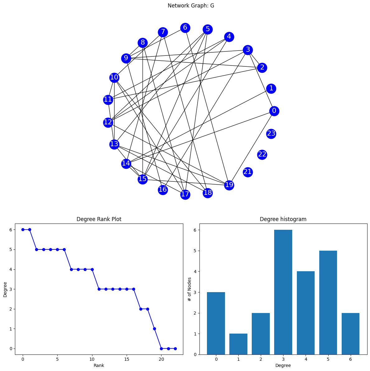
[(0, 3), (1, 1), (2, 3), (3, 5), (4, 3), (5, 4), (6, 2), (7, 3), (8, 3), (9, 5), (10, 5), (11, 4), (12, 4), (13, 6), (14, 5), (15, 6), (16, 2), (17, 4), (18, 3), (19, 5), (21, 0), (22, 0), (23, 0)]
------------------------------ k = 1 -------------------------------
21 0
22 0
23 0
Graph with 20 nodes and 38 edges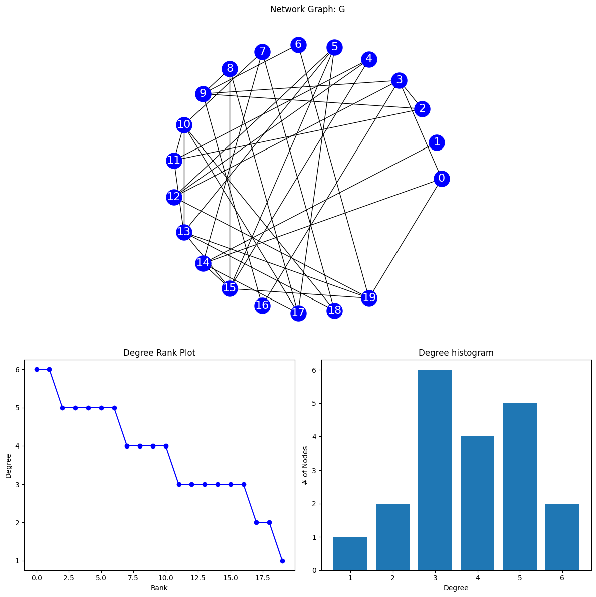
[(0, 3), (1, 1), (2, 3), (3, 5), (4, 3), (5, 4), (6, 2), (7, 3), (8, 3), (9, 5), (10, 5), (11, 4), (12, 4), (13, 6), (14, 5), (15, 6), (16, 2), (17, 4), (18, 3), (19, 5)]
------------------------------ k = 2 -------------------------------
1 1
21 0
22 0
23 0
Graph with 19 nodes and 37 edges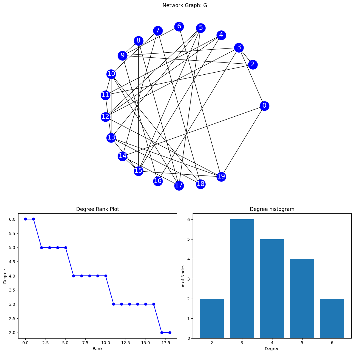
[(0, 3), (2, 3), (3, 5), (4, 3), (5, 4), (6, 2), (7, 3), (8, 3), (9, 5), (10, 5), (11, 4), (12, 4), (13, 6), (14, 4), (15, 6), (16, 2), (17, 4), (18, 3), (19, 5)]
------------------------------ k = 3 -------------------------------
1 1
6 2
16 2
21 0
22 0
23 0
Graph with 17 nodes and 33 edges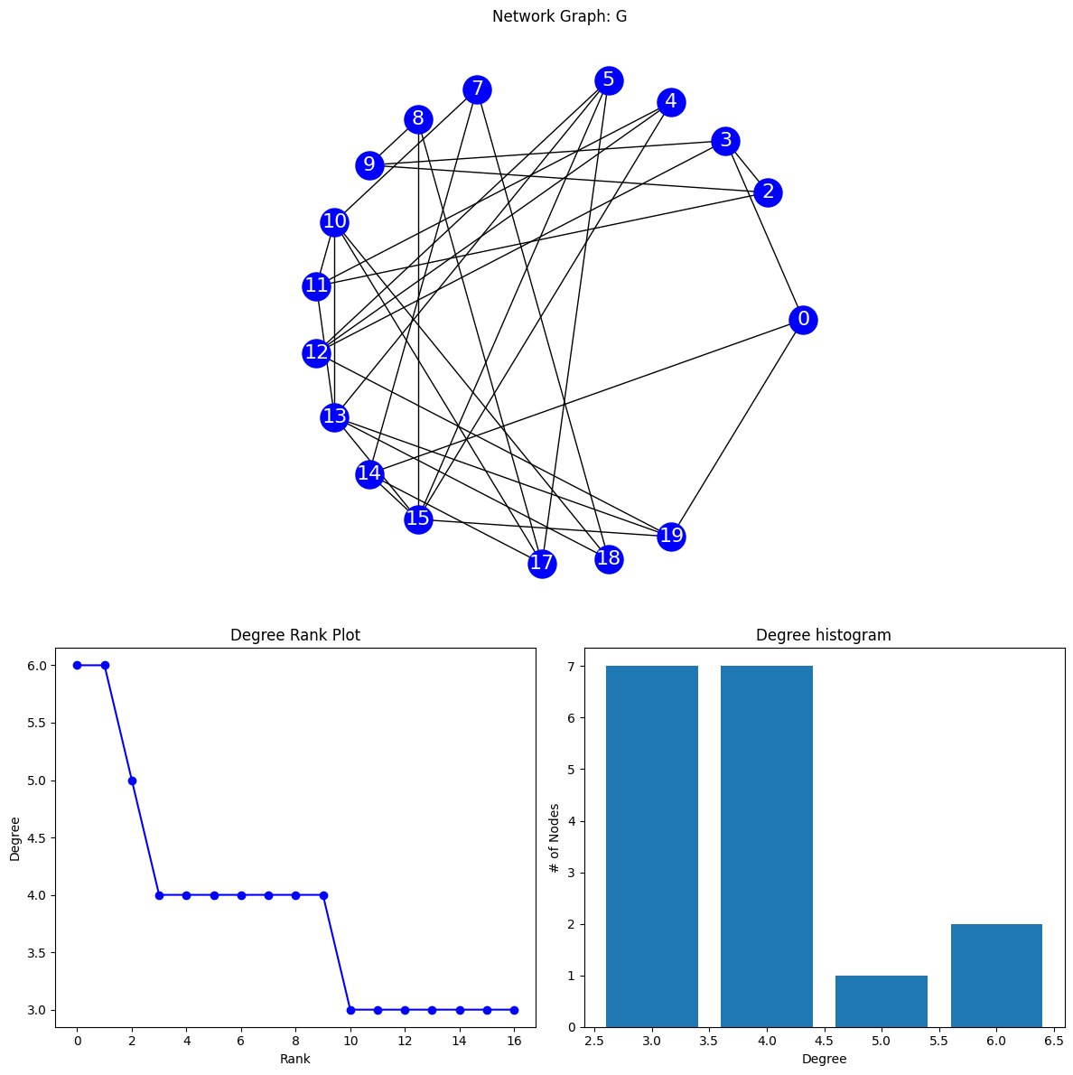
[(0, 3), (2, 3), (3, 4), (4, 3), (5, 4), (7, 3), (8, 3), (9, 3), (10, 5), (11, 4), (12, 4), (13, 6), (14, 4), (15, 6), (17, 4), (18, 3), (19, 4)]
------------------------------ k = 4 -------------------------------
0 3
1 1
2 3
4 3
6 2
7 3
8 3
16 2
18 3
21 0
22 0
23 0
Graph with 11 nodes and 16 edges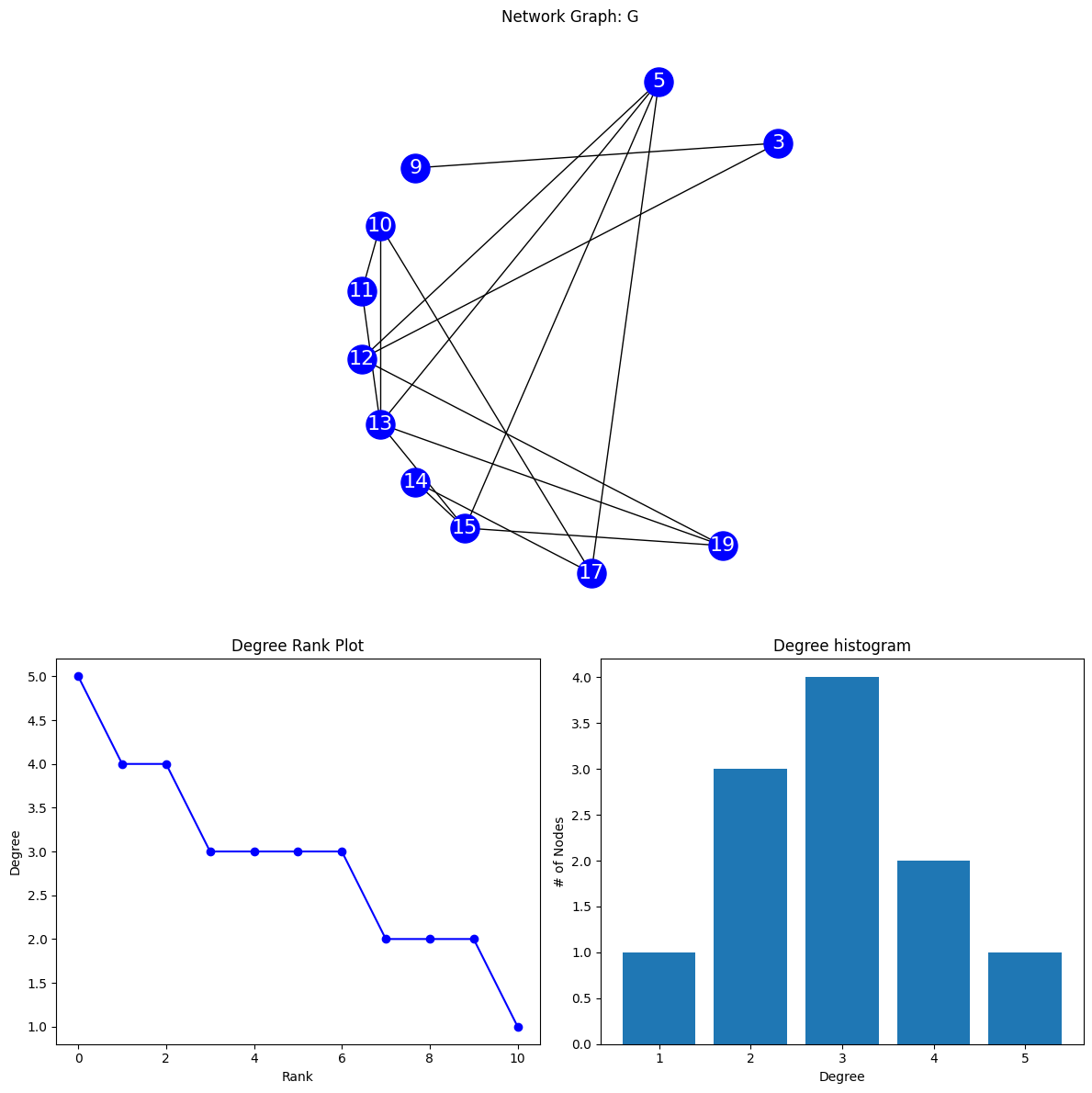
[(3, 2), (5, 4), (9, 1), (10, 3), (11, 2), (12, 3), (13, 5), (14, 2), (15, 4), (17, 3), (19, 3)]References
Disclaimer: This document is not an original work. It contains content from many sources and is for educational purposes only.