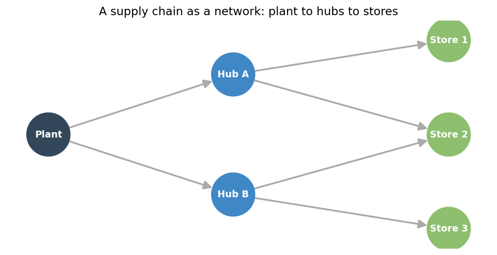
An Introduction to Network Optimization
Flows, Routes, and Structure over Graphs
Motivation and framing
What is network optimization?
- Networks (graphs) describe a system as nodes (points) joined by edges (links)
- nodes: cities, routers, machines, people, tasks
- edges: roads, cables, pipes, assignments, dependencies
- Network optimization = finding the best way to use or shape a network
- best flow: how much to send on each edge (traffic, goods, data)
- best route: which path or paths to follow (navigation, delivery)
- best structure: which edges to build or keep (design, connectivity)
- “Best” is set by an objective (minimize cost or distance, maximize throughput) under constraints (capacities, demands, budgets)
Why networks are a special case
- General optimization can be brutally hard; an arbitrary problem has no shortcut
- Network problems come with extra structure from the graph itself
- conservation: at each node, what flows in must flow out
- sparsity and locality: every constraint touches just a couple of nodes
- Structure buys efficiency: many network problems have fast, exact algorithms
- polynomial time: runtime grows like a power of the input size, not exponentially
- Theme for today: the more structure a problem has, the easier it is to solve
Where it shows up
- Logistics and supply chains: route trucks, place inventory, cut shipping cost
- Telecom and the internet: route packets, provision bandwidth, avoid congestion
- Transportation: shortest routes, traffic assignment, transit planning
- Project scheduling: order dependent tasks, find the critical path
- Matching markets: workers to jobs, students to schools, riders to drivers
- Common thread: a graph, limited resources, and a quantity to optimize
The problem taxonomy
A map of the landscape
- A small set of canonical problems covers most of the field
- Shortest path: cheapest route between two nodes
- Minimum spanning tree (MST): cheapest set of edges connecting everything
- Maximum flow: most throughput from a source to a sink
- Minimum-cost flow: cheapest way to meet supplies and demands
- Assignment / matching: pair up two groups optimally
- Routing (TSP, VRP): visit many locations in the best order
- TSP = traveling salesman problem
- VRP = vehicle routing problem
- Most real problems are variations or combinations of these building blocks
Problems can be easy or very hard
- Two very different types of problems
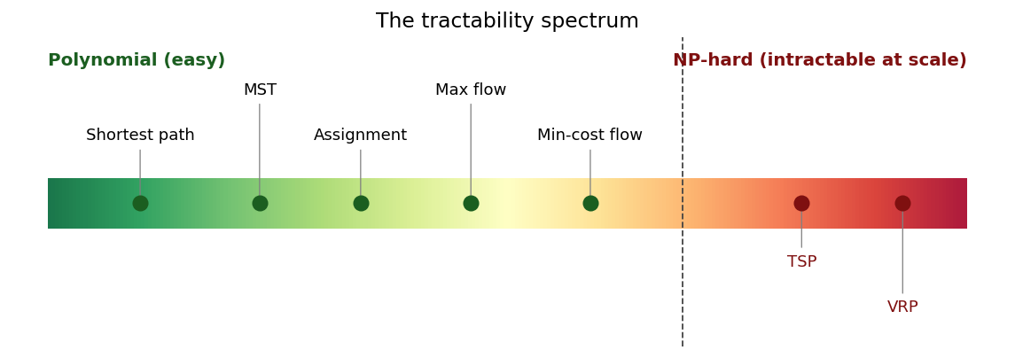
- Polynomial (tractable): shortest path, MST, max flow, min-cost flow, assignment
- solvable exactly and fast, even for very large instances
- NP-hard (intractable at scale): TSP, VRP, many design problems
- no known algorithm solves all instances quickly; we lean on heuristics
- Knowing which side you are on tells you whether to seek the optimum or a good enough answer
What does “NP-hard” mean?
- A problem is NP-hard if it is at least as hard as an entire class of famously difficult problems
- Practical translation:
- no known fast (polynomial) algorithm exists for the worst case
- as the input grows, exact solving can take exponential time
- e.g. of exponential growth: 2^10 = 1024, 2^20 = 1,048,576, 2^30 = 1,073,741,824
- a 10 city tour is trivial; a 60 city tour has more possible routes than there are atoms in the observable universe
- We strongly suspect (but have not proven) that no fast exact method will ever be found
- this is the famous P versus NP question, still open
- Consequence: for NP-hard problems we accept near-optimal answers from heuristics
Problem-1: Shortest path problems
The problem
- Given a graph with edge weights (distances, costs, times), find the path of minimum total weight between two nodes
- Weights need not be physical distance: they can encode money, delay, risk, or fuel
- Applications
- GPS navigation and mapping
- packet routing in networks
- a subroutine inside larger optimizers (flows, matching, scheduling)
Recall: Breadth-first search (BFS)
- BFS: special case of shortest path where all edge weights are equal (unweighted graphs, each edge = 1)
- Minimizes number of edges: “minimum total weight” = “fewest hops”
- FIFO queue ensures first time a node is reached, it’s via shortest path
- Dijkstra = BFS generalized to weighted graphs
- Swaps FIFO queue for priority queue based on total path weight
- With uniform weights, Dijkstra reduces exactly to BFS
- Shortest path algorithm continuum:
- BFS: uniform weights, FIFO queue, \(O(V+E)\)
- 0–1 BFS: weights in {0,1}, deque, \(O(V+E)\)
- Dijkstra: non-negative weights, min-heap, \(O((V+E)\log V)\)
- Bellman–Ford: allows negative weights, \(O(VE)\)
- Takeaway:
- Use BFS when edge weights don’t matter
- Dijkstra is the natural extension when they do: swap the queue for a priority queue
Dijkstra’s algorithm
- The standard method when all edge weights are nonnegative
- Greedy idea: always finalize the closest node you have not settled yet
- keep a tentative distance for every node: source = 0, all others = infinity
- repeatedly pick the unsettled node with the smallest tentative distance and settle it
- relax its outgoing edges: if reaching a neighbor through this node is cheaper, update it
- Why nonnegative weights matter
- once a node is settled, no later path can beat it, since adding more nonnegative edges can only increase cost
- a negative edge breaks this promise: a cheaper detour could appear after settling
Example: setup
- Goal: shortest path from A to E in the graph below
- Rule: at each step, settle the unsettled node with the smallest tentative distance, then relax its edges
- Start: \(d(A) = 0\), and \(d(\cdot) = \infty\) for every other node
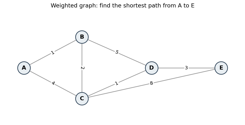
Example: running Dijkstra
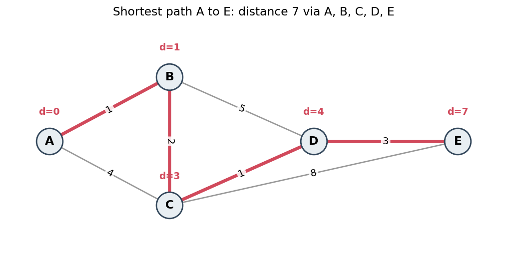
- Settle A (0): relax to \(B = 1\), \(C = 4\)
- Settle B (1): relax \(C = \min(4,\, 1+2) = 3\), and \(D = 1+5 = 6\)
- Settle C (3): relax \(D = \min(6,\, 3+1) = 4\), and \(E = 3+8 = 11\)
- Settle D (4): relax \(E = \min(11,\, 4+3) = 7\)
- Settle E (7): finished
- Result: shortest distance \(A \to E = 7\), via A, B, C, D, E
- Note \(C\) was improved from 4 to 3 before it settled: the greedy pick still allows updates until a node is locked in
Negative edges: Bellman-Ford
- If some weights are negative (rebates, gains), Dijkstra can return a wrong answer
- Bellman-Ford handles negative edges
- it relaxes all edges repeatedly, \(|V| - 1\) times
- it also detects negative cycles: loops you could ride forever to keep lowering cost, which make “shortest path” undefined
- Trade-off: more general than Dijkstra, but slower
Complexity note
- Dijkstra with a binary heap: about \(O\big((V + E)\log V\big)\)
- \(V\) = number of nodes, \(E\) = number of edges
- Bellman-Ford: \(O(V \cdot E)\), slower but more general
- Both are polynomial: shortest path sits firmly in the easy world
Problem-2:Max flow and min cut
Flow networks
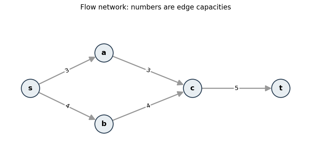
- A flow network is a directed graph with
- a source \(s\) (produces flow) and a sink \(t\) (absorbs flow)
- a capacity on each edge: the most it can carry
- A flow assigns a value to each edge so that
- capacity: edge flow never exceeds its capacity
- conservation: at every node other than \(s\) and \(t\), flow in = flow out
- Max flow problem: push as much as possible from \(s\) to \(t\)
Ford-Fulkerson and augmenting paths
- Augmenting path: a path from \(s\) to \(t\) that still has spare capacity
- Method
- find an augmenting path, then push as much flow as its tightest edge allows
- repeat until no augmenting path remains
- Residual graph is what makes this correct
- for each unit of flow sent on an edge, add a reverse residual edge of the same amount
- reverse edges let the algorithm undo or reroute earlier choices when a better option appears
- When the residual graph has no \(s\) to \(t\) path left, the flow is maximum
Worked example
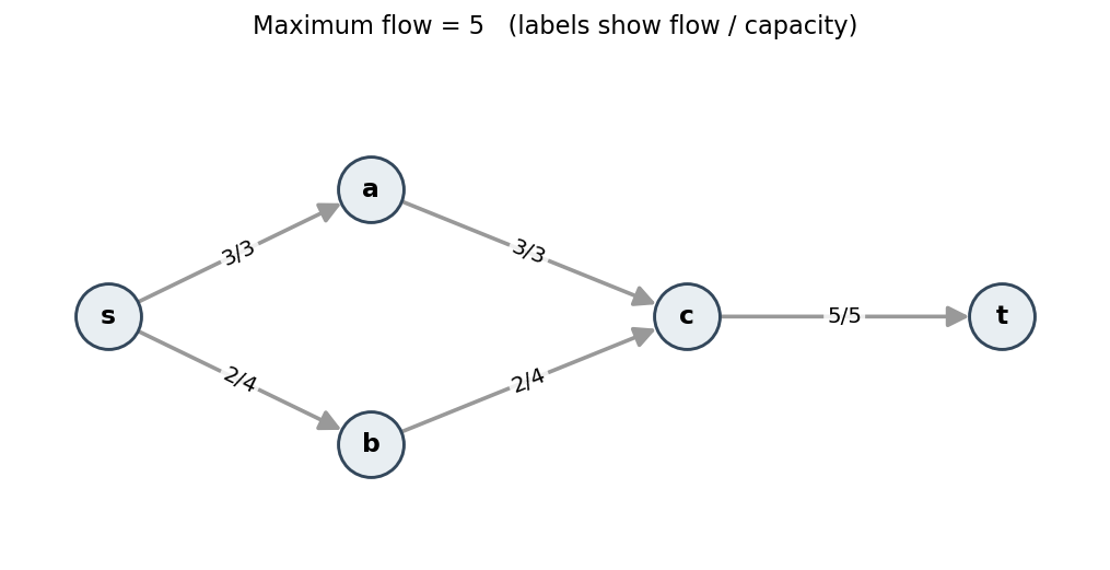
- Capacities: \(s \to a = 3\), \(s \to b = 4\), \(a \to c = 3\), \(b \to c = 4\), \(c \to t = 5\)
- Augment s, a, c, t: tightest edge is 3, push 3
- Augment s, b, c, t: only 2 capacity remains on \(c \to t\), push 2
- No augmenting path is left: every route into \(t\) is now full
- Maximum flow = 5
The max-flow min-cut theorem
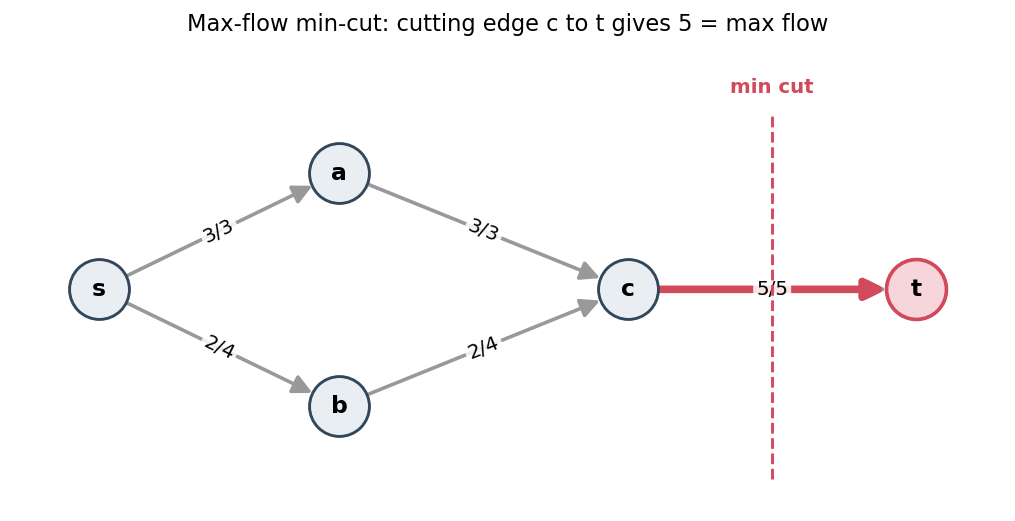
- An s-t cut splits the nodes into two sides, with \(s\) on one and \(t\) on the other
- the cut capacity = total capacity of edges crossing from the \(s\) side to the \(t\) side
- Theorem: the maximum flow equals the minimum cut capacity
- In our example the bottleneck is the single edge \(c \to t\) (capacity 5)
- cutting it separates \(s\) from \(t\), and \(5 =\) the max flow
- Why it matters: this is duality made concrete
- one problem maximizes (flow), its partner minimizes (cut), and they meet exactly
- the min cut pinpoints where the real bottleneck is
The linear programming connection
Network problems as linear programs
- A linear program (LP) optimizes a linear objective subject to linear constraints, with variables allowed to take continuous (fractional) values
- Network problems fit this mold naturally
- variables: how much flow on each edge
- objective: minimize cost, or maximize flow (linear in those variables)
- constraints: capacities and conservation (all linear)
- So shortest path, max flow, and min-cost flow are all special linear programs
Integers “for free”
- Normally, forcing an LP to give whole-number answers is a separate, hard problem (integer programming)
- Network constraint matrices have a special property called total unimodularity (TU)
- loosely: the constraint structure is so clean that the LP’s corner solutions are always integer points
- Consequence: if capacities and supplies are integers, the LP optimum is automatically integer
- no integer constraints, no rounding, no branch and bound needed
- This is why you can plan to ship 3 trucks, not 3.4 trucks, and still solve it as a fast LP
Min-cost flow: the unifying model
- Min-cost flow: route the required supply to meet demand at minimum total cost, while respecting capacities
- It specializes to the other problems
- shortest path: send one unit from \(s\) to \(t\), with edge cost = weight
- max flow: set costs to zero and maximize units pushed within capacities
- assignment: bipartite supplies and demands of one unit each
Master min-cost flow and you get a whole family of problems at once
Example: Network to Linear Program
The Scenario
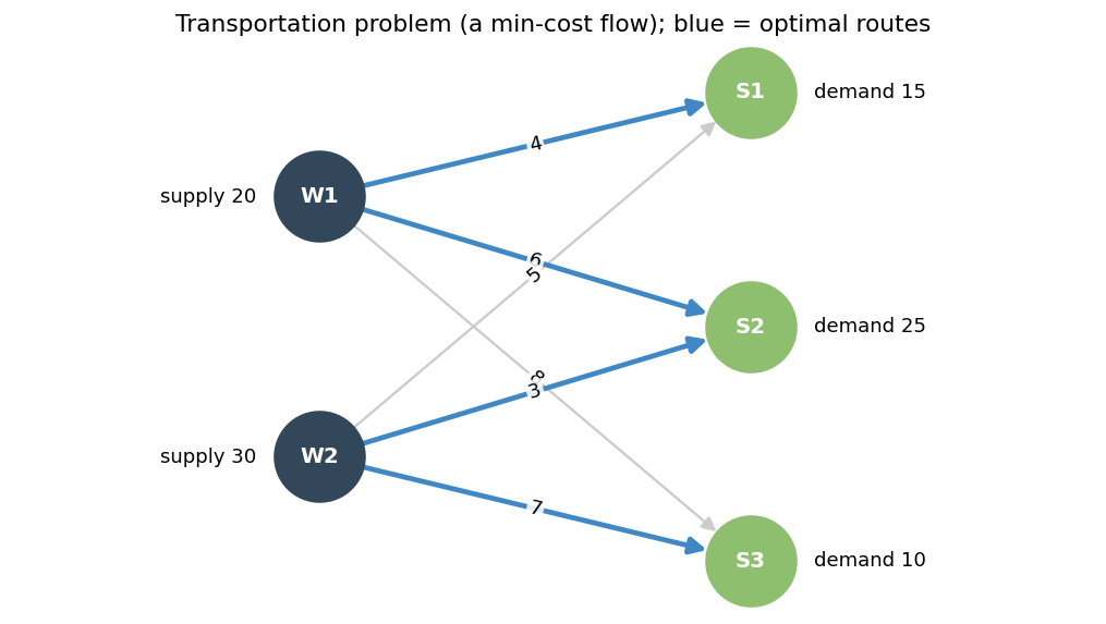
- Picture two warehouses on the left and three stores on the right, with a shipping route drawn from every warehouse to every store
- Supply (units available): W1 = 20, W2 = 30
- Demand (units required): S1 = 15, S2 = 25, S3 = 10
- Each route has a per-unit cost and a capacity of 20 units
| cost per unit | S1 | S2 | S3 |
|---|---|---|---|
| W1 | 4 | 6 | 8 |
| W2 | 5 | 3 | 7 |
- Total supply \(= 50 =\) total demand, so the problem is balanced: every unit must move
- Goal: meet all demand at the least total shipping cost
Jargon translation
- The trick is a one-to-one mapping from network language to LP language
| Network world | LP world |
|---|---|
| a shipping route | a decision variable |
| per-unit route cost | a cost coefficient in the objective |
| a warehouse’s supply | a “ships out its supply” equation |
| a store’s demand | a “receives its demand” equation |
| a route’s capacity | an upper bound on that variable |
| no negative shipments | nonnegativity, a lower bound of 0 |
- Work down this table row by row and the LP writes itself
Step 1: Decision Variables
- What do we actually control? The units sent on each route
- Let \(x_{ij} =\) units shipped from warehouse \(i\) to store \(j\)
- Six routes, so six variables:
- from W1: \(x_{11}, \; x_{12}, \; x_{13}\)
- from W2: \(x_{21}, \; x_{22}, \; x_{23}\)
- Everything else (costs, supplies, demands) is fixed data, not a variable
- These six numbers are the only knobs the solver gets to turn
Step 2: The Objective
- We pay \(c_{ij}\) for each unit on route \((i, j)\), so that route costs \(c_{ij}\, x_{ij}\)
- Total cost is just the sum over all routes, and we want it as small as possible:
\[\min \; Z = 4x_{11} + 6x_{12} + 8x_{13} + 5x_{21} + 3x_{22} + 7x_{23}\]
- Compactly, \(\min \; Z = \sum_{i}\sum_{j} c_{ij}\, x_{ij}\)
- Every coefficient is read straight off the cost table, nothing more
Step 3: Supply Constraints
- Rule: everything leaving a warehouse must add up to its supply
- Read each row of the cost table left to right, and set the sum equal to that warehouse’s supply:
- W1: \(\quad x_{11} + x_{12} + x_{13} = 20\)
- W2: \(\quad x_{21} + x_{22} + x_{23} = 30\)
- Why equality and not \(\le\)? Because the problem is balanced, so no supply can sit idle
- if supply exceeded demand, these would relax to \(\le\)
Step 4: Demand Constraints
- Rule: everything arriving at a store must add up to its demand
- Read each column of the cost table top to bottom, and set the sum equal to that store’s demand:
- S1: \(\quad x_{11} + x_{21} = 15\)
- S2: \(\quad x_{12} + x_{22} = 25\)
- S3: \(\quad x_{13} + x_{23} = 10\)
- Mirror image of supply: rows feed the supply equations, columns feed the demand equations
Step 5: Capacity and Nonnegativity
- Capacity: no single route may carry more than 20 units
- Nonnegativity: you cannot ship a negative quantity
- Both fold into simple bounds on each variable:
\[0 \le x_{ij} \le 20 \quad \text{for every route } (i, j)\]
- In
linprogthese become theboundslist, one \((\text{low}, \text{high})\) pair per variable
The Complete Linear Program
- Stacking Steps 1 through 5 gives the full model:
\[ \begin{aligned} \min_{x} \quad & 4x_{11} + 6x_{12} + 8x_{13} + 5x_{21} + 3x_{22} + 7x_{23} \\ \text{s.t.} \quad & x_{11} + x_{12} + x_{13} = 20 && \text{(W1 supply)} \\ & x_{21} + x_{22} + x_{23} = 30 && \text{(W2 supply)} \\ & x_{11} + x_{21} = 15 && \text{(S1 demand)} \\ & x_{12} + x_{22} = 25 && \text{(S2 demand)} \\ & x_{13} + x_{23} = 10 && \text{(S3 demand)} \\ & 0 \le x_{ij} \le 20 && \text{for all } i, j \end{aligned} \]
- 6 variables, 5 equality constraints, box bounds: a complete, solvable LP
- Nuance: one of the five equations is redundant, since the supply totals and demand totals both equal 50, but leaving it in does no harm
The Same LP as Matrices
linprogdoes not read sentences, it reads arrays, so line the constraints up with variables as columns and constraints as rows:
\[ \underbrace{\begin{bmatrix} 1 & 1 & 1 & 0 & 0 & 0 \\ 0 & 0 & 0 & 1 & 1 & 1 \\ 1 & 0 & 0 & 1 & 0 & 0 \\ 0 & 1 & 0 & 0 & 1 & 0 \\ 0 & 0 & 1 & 0 & 0 & 1 \end{bmatrix}}_{A_{eq}} \begin{bmatrix} x_{11} \\ x_{12} \\ x_{13} \\ x_{21} \\ x_{22} \\ x_{23} \end{bmatrix} = \underbrace{\begin{bmatrix} 20 \\ 30 \\ 15 \\ 25 \\ 10 \end{bmatrix}}_{b_{eq}} \]
- Each entry is just 1 if the route touches that warehouse or store, else 0
- That clean 0/1 pattern is special: it guarantees whole-number answers with no extra effort
Code demo
What we will build
- A tiny transportation problem, the classic min-cost flow
- 2 warehouses with supply, 3 stores with demand
- a per-unit shipping cost on each route, plus a capacity per route
- We solve it two ways and confirm they agree
- a graph solver (NetworkX min-cost flow)
- a linear program (SciPy
linprog), which shows the “integer for free” property
- Design note: the whole instance lives in a
CONFIGdictionary, so it is easy to edit, reuse, or feed into a parameter search
# The full problem instance lives in CONFIG so it is easy to modify,
# reuse, or sweep over later (for example in a parameter search).
CONFIG = {
    "supply": {"W1": 20, "W2": 30},              # units available at each warehouse
    "demand": {"S1": 15, "S2": 25, "S3": 10},    # units required at each store
    "cost": {                                    # per-unit shipping cost per route
        ("W1", "S1"): 4, ("W1", "S2"): 6, ("W1", "S3"): 8,
        ("W2", "S1"): 5, ("W2", "S2"): 3, ("W2", "S3"): 7,
    },
    "edge_capacity": 20,                         # max units allowed on any route
}

# A balanced transportation problem needs total supply == total demand.
assert sum(CONFIG["supply"].values()) == sum(CONFIG["demand"].values())
print("total supply:", sum(CONFIG["supply"].values()))
print("total demand:", sum(CONFIG["demand"].values()))
total supply: 50
total demand: 50Anatomy of a linprog call
Standard form: linprog always solves the same shape of problem - minimize \(c^\top x\) - subject to \(A_{ub}\, x \le b_{ub}\), then \(A_{eq}\, x = b_{eq}\), and \(l \le x \le u\)
Inputs (each is a plain list or NumPy array) - \(c\): 1-D cost vector, length = number of variables - \(A_{ub}\), \(b_{ub}\): matrix and vector for the inequality (\(\le\)) constraints - \(A_{eq}\), \(b_{eq}\): matrix and vector for the equality (\(=\)) constraints - bounds: a list of \((\text{low}, \text{high})\) pairs, one per variable (default \((0, \infty)\)) - method: the solver to use, default "highs"
Output: a single OptimizeResult object - .x: the optimal solution vector (the variable values) - .fun: the optimal objective value \(c^\top x\) - .success: True if an optimum was found - .status, .message: why it stopped (0 = solved, 2 = infeasible, 3 = unbounded) - .slack, .con: leftover room in the inequality and equality constraints
Key idea: everything is just vectors and matrices - variable \(j\) is column \(j\) in every matrix, so all arrays must line up - this uniform layout is what makes an LP fast to solve and easy to build programmatically
Solve with a network solver
- NetworkX convention: a node’s
demandis negative for supply (produces flow) and positive for demand (absorbs flow) - We build the directed graph from
CONFIG, then callmin_cost_flow
import networkx as nx

G = nx.DiGraph()
for warehouse, supply in CONFIG["supply"].items():
    G.add_node(warehouse, demand=-supply)     # negative demand == supply
for store, demand in CONFIG["demand"].items():
    G.add_node(store, demand=demand)          # positive demand == requirement
for (u, v), unit_cost in CONFIG["cost"].items():
    G.add_edge(u, v, weight=unit_cost, capacity=CONFIG["edge_capacity"])

flow = nx.min_cost_flow(G)                    # optimal units on every edge
total_cost = nx.cost_of_flow(G, flow)

print("optimal shipping cost:", total_cost)
for u in flow:
    for v, units in flow[u].items():
        if units > 0:
            print(f"  ship {units:>2} units   {u} -> {v}")
optimal shipping cost: 220
ship 15 units W1 -> S1
ship 5 units W1 -> S2
ship 20 units W2 -> S2
ship 10 units W2 -> S3Solve as a linear program
- Same problem, now written as an LP with variables $x_{uv} = $ units shipped on route \((u, v)\)
- Objective: \(\min \sum_{(u,v)} c_{uv}\, x_{uv}\)
- Constraints: each warehouse ships its full supply, each store receives its full demand
- We never ask for integers, yet total unimodularity delivers them anyway
import numpy as np
from scipy.optimize import linprog

routes = list(CONFIG["cost"].keys())
cost_vector = [CONFIG["cost"][r] for r in routes]

# Equality constraints: supply out of each warehouse, demand into each store.
A_eq, b_eq = [], []
for warehouse, supply in CONFIG["supply"].items():
    A_eq.append([1.0 if u == warehouse else 0.0 for (u, v) in routes])
    b_eq.append(supply)
for store, demand in CONFIG["demand"].items():
    A_eq.append([1.0 if v == store else 0.0 for (u, v) in routes])
    b_eq.append(demand)

bounds = [(0, CONFIG["edge_capacity"]) for _ in routes]   # continuous, not integer
result = linprog(cost_vector, A_eq=A_eq, b_eq=b_eq, bounds=bounds, method="highs")

print("LP optimal cost:", result.fun)
print("solution is integer without asking:",
      np.allclose(result.x, np.round(result.x)))
for (u, v), units in zip(routes, np.round(result.x, 6)):
    if units > 0:
        print(f"  ship {units:g} units   {u} -> {v}")
LP optimal cost: 220.0
solution is integer without asking: True
ship 15 units W1 -> S1
ship 5 units W1 -> S2
ship 20 units W2 -> S2
ship 10 units W2 -> S3Final case: when problems get hard
TSP and VRP
- Traveling Salesperson Problem (TSP): visit every city exactly once and return home, at minimum total distance
- Vehicle Routing Problem (VRP): TSP with multiple vehicles, capacities, and time windows, the real logistics problem
- Both are NP-hard: no known fast exact algorithm at scale
- In practice we use heuristics and approximations
- nearest neighbor, 2-opt local search, metaheuristics, modern solvers
- the goal shifts from provably optimal to very good, very quickly
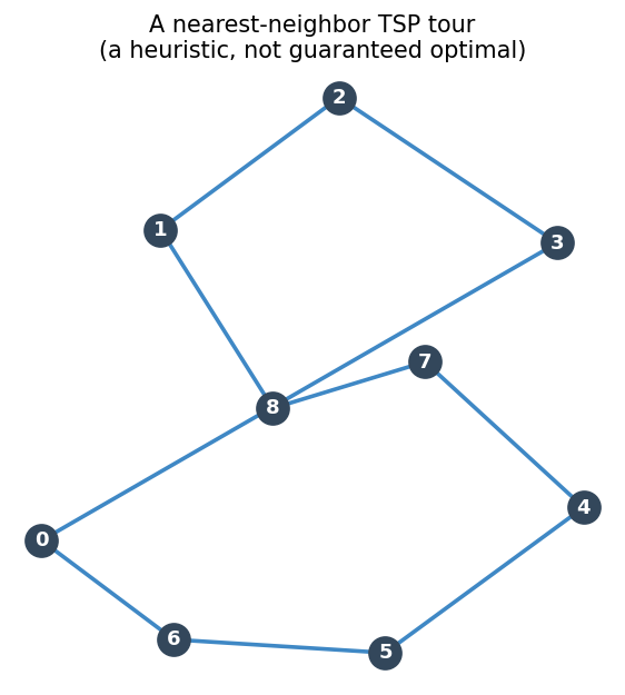
The tractability spectrum
- Easy (polynomial): solve exactly at scale
- shortest path, MST, max flow, min-cost flow, assignment
- Hard (NP-hard): solve approximately at scale
- TSP, VRP, and many network design problems
- The dividing line is structure: conservation and total unimodularity are what make the easy problems easy
- Practical instinct: first try to model your problem as min-cost flow, and only reach for heuristics when you truly cannot
Where to go next
- Algorithms in depth: heaps for Dijkstra, faster max-flow methods (Dinic, push-relabel)
- Duality and LP theory: the general engine behind min-cut and much more
- Integer programming: what to do when total unimodularity does not save you
- Heuristics and metaheuristics: local search, simulated annealing, tabu search
- Tools: NetworkX and SciPy for learning, industrial solvers (OR-Tools, Gurobi) for production
Summary
- Both methods return the same optimal cost and the same integer shipments
- The LP was never told to use integers, yet it produced them: total unimodularity at work
- The
CONFIGpattern makes this a clean starting point for real work- swap in real costs, capacities, and supplies
- wrap the solver in a loop to search over scenarios or tune parameters
- From here you grow toward production: more nodes, side constraints, and industrial solvers, all resting on the same min-cost flow foundation