Linear programming
Motivation
Linear programming is a mathematical method for optimizing a linear objective function subject to linear equality and inequality constraints.
Examples:
- Minimum-Cost Flow: LP minimizes total cost while satisfying flow conservation and capacity constraints.
- Multi-Commodity Flow: LP handles multiple flows sharing the same network under linear constraints.
- Assignment and Transportation Problems: Special cases of LP used in resource allocation on networks.
These problems are typically modeled with:
- Linear objective functions (e.g., minimize total cost)
- Linear equality/inequality constraints (e.g., flow conservation, capacity limits)
Linear equations
Quick detour
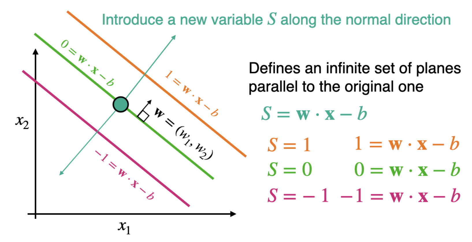
Recall: Equations of planes in higher dimensions
Equation of a Plane in 2D: - A line in 2D can be written as:
\[ a x_1+b x_2+c=0 \]
- \(a, b\) define the direction of the line; \(c\) is the offset.
Equation of a Plane in 3D:
- A plane in 3D is given by:
\[ a x_1+b x_2+c x_3+d=0 \]
- The normal vector \((a, b, c)\) defines the plane’s orientation.
Equation of a Hyperplane in N-D Space:
- General form in \(N\)-dimensional space:
\[ w_1 x_1+w_2 x_2+\cdots+w_N x_N+b=0 \]
\({ }^{-} w\) is the normal vector, \(b\) is the bias term. - Separates \(N\)-dimensional space into two half-spaces.
Normal vector
The equation of a plane in 3D can be written using the normal vector \(\vec{n}=\langle a, b, c\rangle\) and a point on the plane \(P_0=\left(x_0, y_0, z_0\right)\) as:
\[ a\left(x-x_0\right)+b\left(y-y_0\right)+c\left(z-z_0\right)=0 \]
Alternatively, in expanded form:
\[ a x+b y+c z=d \]
where: - \(a, b, c\) are the components of the normal vector \(\vec{n}\), - \(d=a x_0+b y_0+c z_0\) is a constant determined by the point on the plane.
Finally, using dot product notation, the equation of a plane in 3D can be written as:
\(\vec{n} \cdot (\vec{r} - \vec{r}_0) = 0\)
Where:
- \(\vec{n} = \langle a, b, c \rangle\) is the normal vector to the plane,
- \(\vec{r} = \langle x, y, z \rangle\) is a position vector to any point on the plane,
- \(\vec{r}_0 = \langle x_0, y_0, z_0 \rangle\) is the position vector of a known point on the plane.
This form expresses that the vector from \(\vec{r}_0\) to \(\vec{r}\) is orthogonal to the normal vector \(\vec{n}\), hence lies in the plane.
Example
Linear programming
Introduction and statement of problem
General constrained optimization problem
An constrained optimization problem involves finding the values of decision variables that minimize (or maximize) an objective function, subject to a set of constraints:
Minimize: \[ f(x_1, x_2, \ldots, x_n) \] Subject to: \[ \begin{aligned} g_1(x_1, x_2, \ldots, x_n) &\;\; \{=,\; \leq,\; \geq\} \;\; b_1 \\ g_2(x_1, x_2, \ldots, x_n) &\;\; \{=,\; \leq,\; \geq\} \;\; b_2 \\ \vdots \\ g_m(x_1, x_2, \ldots, x_n) &\;\; \{=,\; \leq,\; \geq\} \;\; b_m \end{aligned} \]
Linear Programming: Overview
- Definition: Linear programming (LP) is a mathematical method for optimizing a linear objective function.
- Constraints: Subject to linear equality and inequality constraints.
- Variables: Decision variables represent quantities to be determined.
- Objective: Maximizes or minimizes the objective function.
- Applications: Used in resource allocation, network optimization, production scheduling, and logistics.
Linear Programming: Statement of problem
- Linear Programming (LP) is a special case of general optimization where both the objective function and all constraints are linear.
- Objective Function Example:
\[ f\left(x_1, x_2, \ldots, x_n\right)=c_1 x_1+c_2 x_2+\ldots+c_n x_n \]
- Constraints Example:
\[ \begin{aligned} a_{11} x_1+a_{12} x_2+\ldots+a_{1 n} x_n & \leq b_1 \\ a_{21} x_1+a_{22} x_2+\ldots+a_{2 n} x_n & \geq b_2 \\ \vdots & \\ x_i & \geq 0 \text { (non-negativity) } \end{aligned} \]
- “Programming” \(\neq\) Coding
- The word programming here refers to planning or scheduling, not computer programming.
- Goal: Choose decision variables to optimize a linear objective while satisfying all linear constraints-yielding the best feasible solution.
- Non-Negativity Constraints: These reflect real-world limits: quantities like time, resources, flow typically cannot be negative.
Visualizing the problem
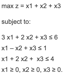
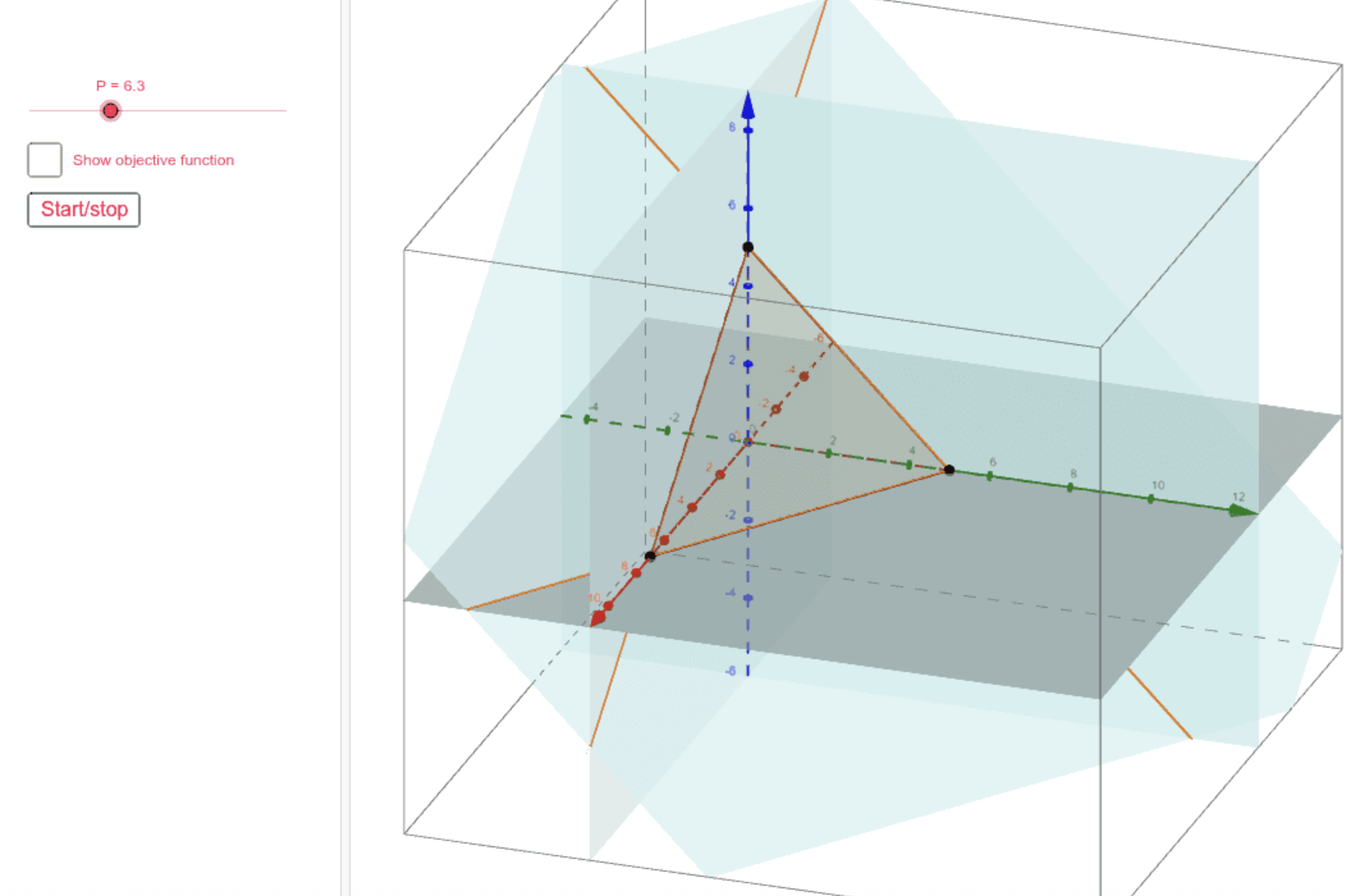
We can visualize the objective contours as planes. Using the objective z = x1 + x2 + x3, we can plot the contours z = 1.5, z = 2.5 (solving each equation for x3 and plotting the surface):
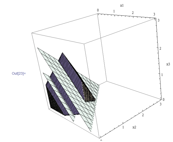

Source: https://greenor.wordpress.com/2014/02/09/visualizing-lps-in-mathematica/
Example: Statement of problem
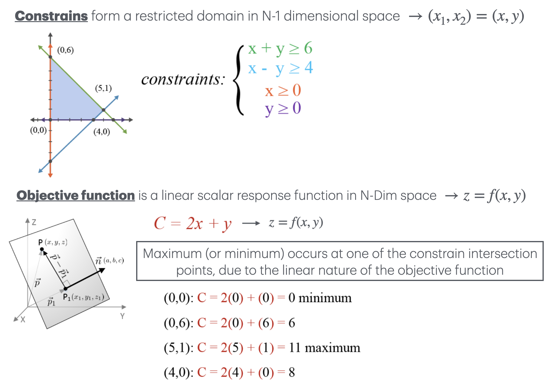
Simple example
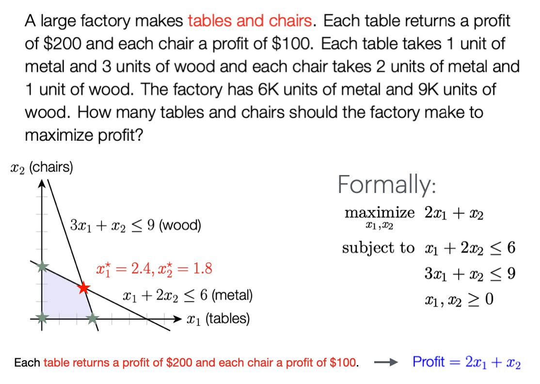
Polytope in 2D
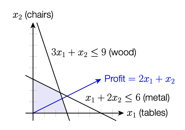
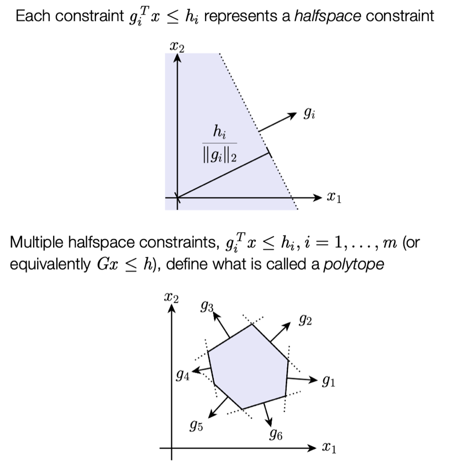
A polytope is the bounded region formed by the intersection of a finite number of linear inequalities.
In \(\mathbb{R}^n\), it is a convex, multi-faced geometric object—a polygon in 2D, a polyhedron in 3D, and higher-dimensional analogs beyond.
It is the blue region in the image below
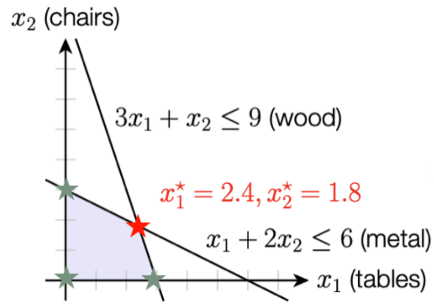
Polytope in 3D
A closed feasible region of a problem with three variables is a convex polyhedron.
The surfaces giving a fixed value of the objective function are planes (not shown).
The linear programming problem is to find a point on the polyhedron that is on the plane with the highest possible value.
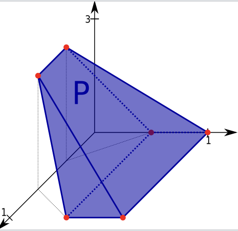
If the problem had more independent variables, e.g. 3, the polytope would have higher dimension
Direction of maximum increase of objective function
- can be obtained by computing the gradient of the objective function \(\nabla \text{Profit}=\nabla P = \left( \frac{\partial P}{\partial x_1},\frac{\partial P}{\partial x_2} \right)= (2,1)\)
General Form of a Linear Program
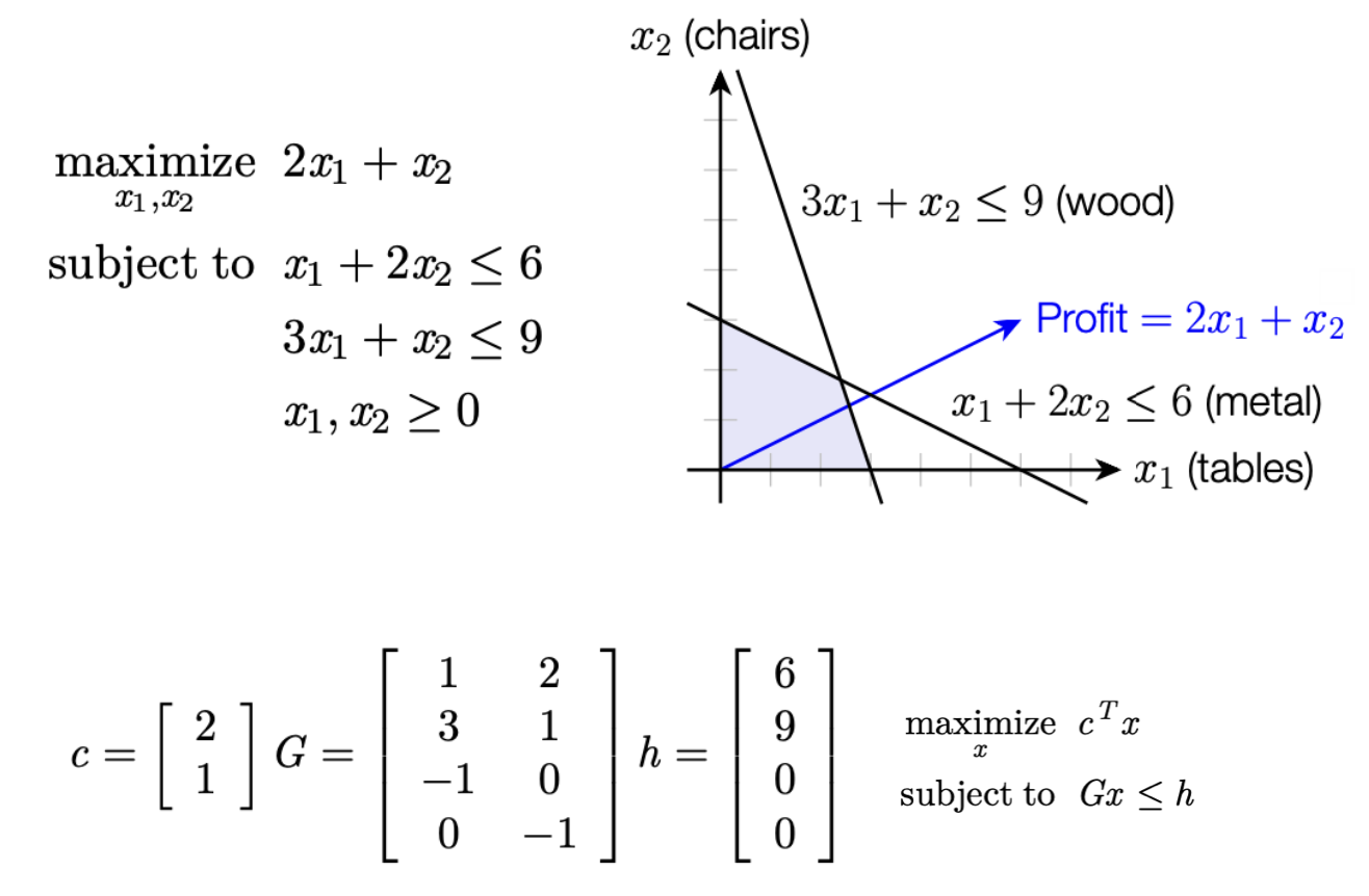
Using linear algebra notation, a linear programming (LP) problem can be written compactly as:
\(\begin{aligned} \underset{x}{\text{maximize}} \quad & c^T x \\ \text{subject to} \quad & Gx \leq h \end{aligned}\)
Symbol Definitions
- \(x \in \mathbb{R}^n\): the optimization variable, an \(n\)-dimensional vector
- \(c \in \mathbb{R}^n\): the cost (or objective) vector
- \(G \in \mathbb{R}^{m \times n}\): the constraint matrix (each row corresponds to one inequality constraint)
- \(h \in \mathbb{R}^m\): the constraint bound vector
- \(c^T x\): the objective function to maximize (dot product of \(c\) and \(x\))
- \(Gx \leq h\): elementwise inequality, meaning each row satisfies \(g_i^T x \leq h_i\)
Note on Equality Constraints
Equality constraints can be expressed using two inequalities:
\(g_i^T x = h_i \;\equiv\; \begin{cases} g_i^T x \leq h_i \\ -g_i^T x \leq -h_i \end{cases}\)
This allows all constraints to be handled uniformly in matrix form.
Example: inequality form
Standard form linear programs
- As a final step toward the solution linear programs, we consider linear programs in a slightly different form
Standard form linear program
\[ \begin{aligned} \underset{x}{\operatorname{minimize }} \, c^T x \\ \text { subject to } & A x=b \\ & x \geq 0 \end{aligned} \]
- where \(x \in \mathbb{R}^n\) is optimization variable
- \(c \in \mathbb{R}^n, A \in \mathbb{R}^{m \times n}\) and \(b \in \mathbb{R}^m\) are problem data ( \(m\) and \(n\) are new dimensions unrelated to the problem dimensions in inequality form);
- also a few technical conditions, like \(A\) should have full row rank, that we won’t dwell or
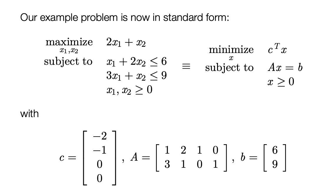
Although they look different, easy to transform between inequality form and standard form
Example: Standard form
Geometry of linear programs
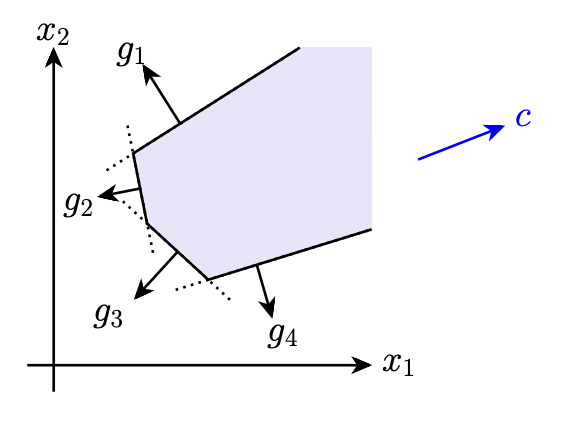
- Linear programming is equivalent to maximizing some direction \(\left(c^T x\right)\) over a polytope
- Important point: note that a maximum will always occur at a “corner” of the polytope
Unbounded and infeasible problems
- Note that a linear program could be set up such that we could obtain infinite objective
- This occurs if the polytope is unbounded in a direction of increasing \(c\)
Solving the LP problem
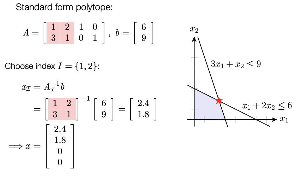
Finding “corners” in standard form polytope
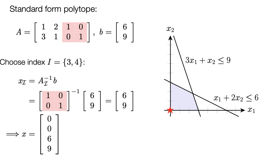
In standard form we assume \(n>m\), so \(A x=b\) is an underdetermined system of equations (more variables than equations)
We can find solutions by selecting a subset of \(m\) columns of \(A\), solving the linear system, and setting remaining \(n-m\) variables to be 0
Those solutions that also satisfy \(x \geq 0\) are the corners of the polytope
Aside: set notation for vectors/matrices
Some set notation will make the resulting systems easier to write
We let \(\mathcal{I} \subseteq\{1, \ldots, n\}\) denote an ordered index set, and let \(\mathcal{I}_i\) the denote the \(i\) th element in set \[ \mathcal{I}=\left\{\mathcal{I}_1, \mathcal{I}_2, \ldots \mathcal{I}_m\right\} \] where \(|\mathcal{I}|=m\) denotes the length of the index set Unlike typical sets order is relevant, so that \(\mathcal{I}=\{1,5\}\) and \(\mathcal{I}=\{5,1\}\) are distinguished between (not important for basic algorithm, but it will be important when we talk about faster versions)
For a vector \(x \in \mathbb{R}^n\) and index set \(\mathcal{I}, x_{\mathcal{I}} \in \mathbb{R}^m\) is a vector of entries selected by indices in \(\mathcal{I}\) \[ x_{\mathcal{I}}=\left[\begin{array}{c} x_{\mathcal{I}_1} \\ x_{\mathcal{I}_2} \\ \vdots \\ x_{\mathcal{I}_m} \end{array}\right] \]
For a matrix \(A \in \mathbb{R}^{m \times n}, A_{\mathcal{I}} \in \mathbb{R}^{m \times m}\) is a matrix where columns are selected by \(\mathcal{I}\) \[ A=\left[\begin{array}{ccc} \mid & \mid & \mid \\ a_{\mathcal{I}_1} & a_{\mathcal{I}_2} \cdots & a_{\mathcal{I}_m} \\ \mid & \mid & \mid \end{array}\right] \]
Naive linear programming algorithm
- For each length- \(m\) subject \(\mathcal{I} \subseteq\{1, \ldots, n\}\) :
- Compute \(x_{\mathcal{I}}=A_{\mathcal{I}}^{-1} b\), and set \(x_j=0\) for \(j \notin \mathcal{I}\)
- If \(x \geq 0\), compute objective \(c^T x\)
- Return \(x\) with lowest computed objective
- But, this requires testing \(\binom{n}{m}=O\left(n^m\right)\) different subsets \(\mathcal{I}\)
The simplex methodis a way of speeding up this “corner finding” process substantially
Example: polytope corners
Example: polytope corners
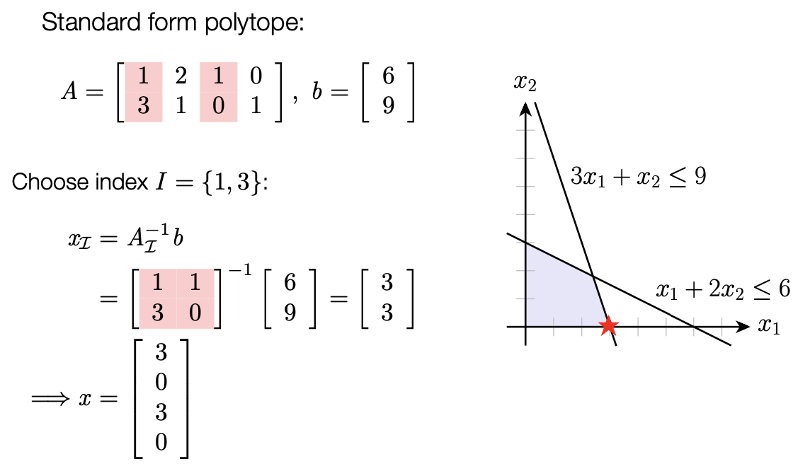
Example: polytope corners
Simplex algorithm
Overview: Simplex algorithm
- Basic idea of simplex algorithm: move along edges of polytope from corner to corner, in directions of decreasing cost
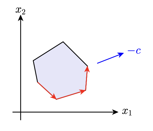
- Exponential complexity in the worst case (need to check a number of corners that is exponential in \(n-m\) ), but it has notable advantages over even the best polynomial time linear programming algorithms (interior point primal-dual methods)
Algorithm steps
- Initialization: Start with an initial feasible solution.
- Objective Function: Identify the entering variable with the most negative coefficient in the objective row.
- Pivot Selection: Choose the leaving variable based on the minimum ratio test.
- Pivot Operation: Update the tableau to reflect new basic variables.
- Iterate: Repeat the process until all coefficients in the objective row are non-negative.
- Optimal Solution: The current solution is optimal when no further improvements can be made. –>
Summary of simplex method
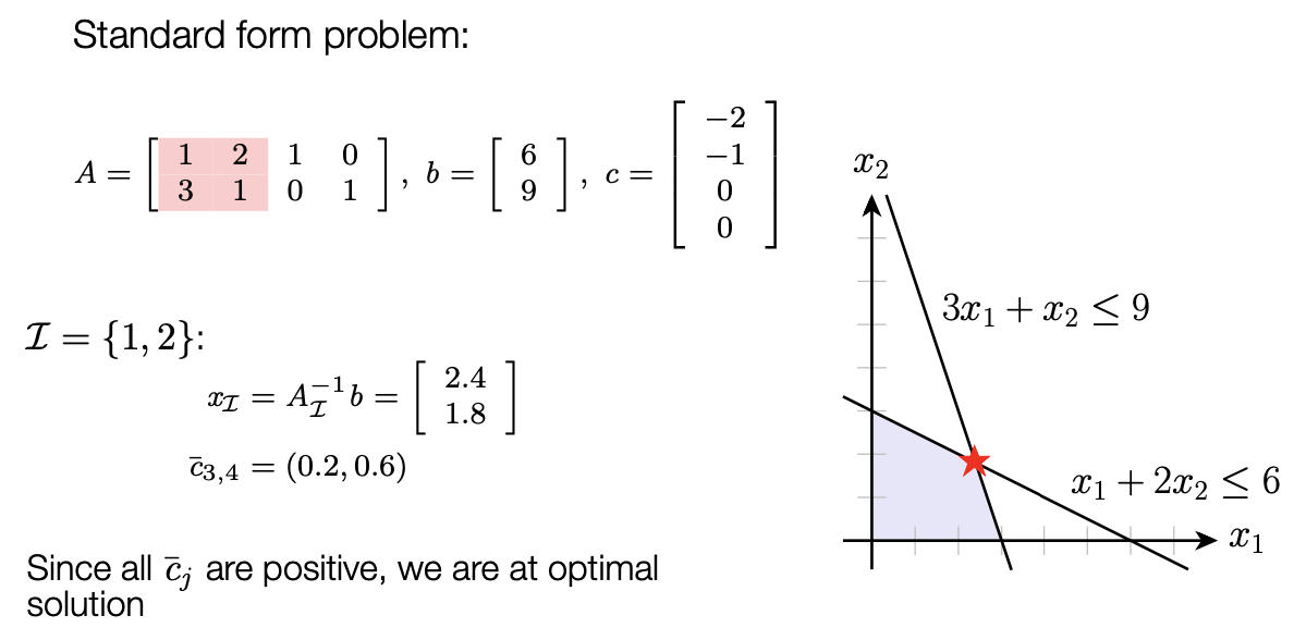
Repeat: 1. Given index set \(\mathcal{I}\) such that \(x_{\mathcal{I}}=A_{\mathcal{I}}^{-1} b \geq 0\) 2. Find \(j\) for which \(\bar{c}_j=c_j-c_{\mathcal{I}}^T A_{\mathcal{I}}^{-1} a_j<0\) (if non exists, return \(\left.x_{\mathcal{I}}^{\star}=A_{\mathcal{I}}^{-1} b\right)\) 3. Compute step direction \(d_{\mathcal{I}}=-A_{\mathcal{I}}^{-1} a_j\) and determine index to remove (or return unbounded if \(d \geq 0\) ) \[ i^{\star}=\underset{i \in \mathcal{I}: d_i<0}{\operatorname{argmin}}-x_i / d_i \] 4. Update index set \[ \mathcal{I} \leftarrow \mathcal{I}-\left\{i^{\star}\right\} \cup\{j\} \]
Illustration of simplex-1
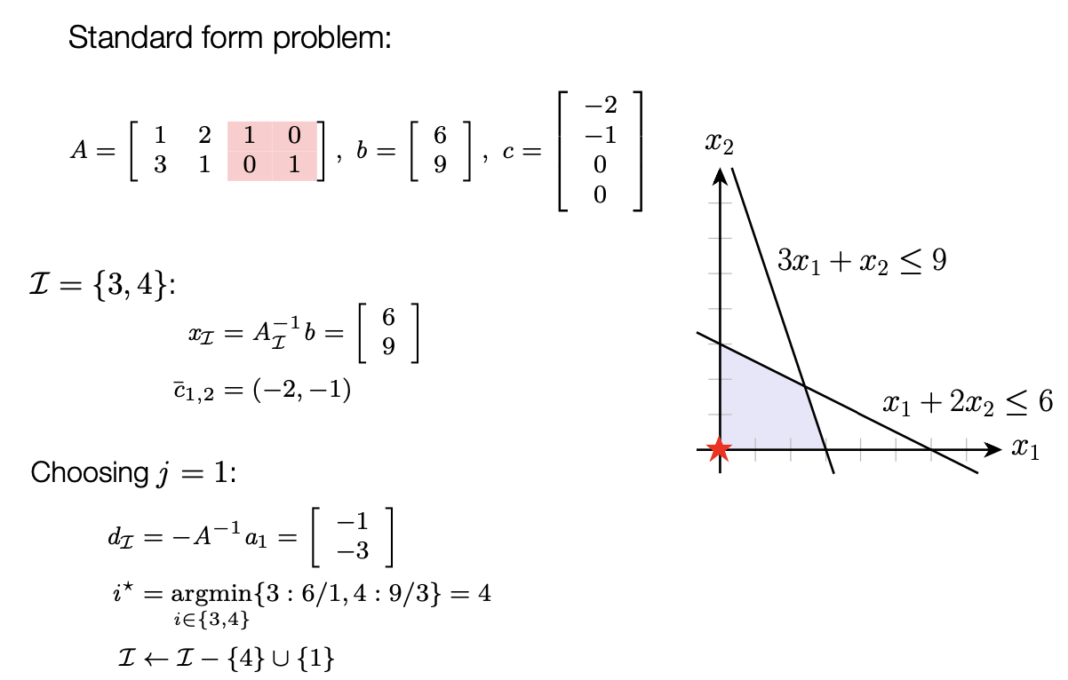
Illustration of simplex-2
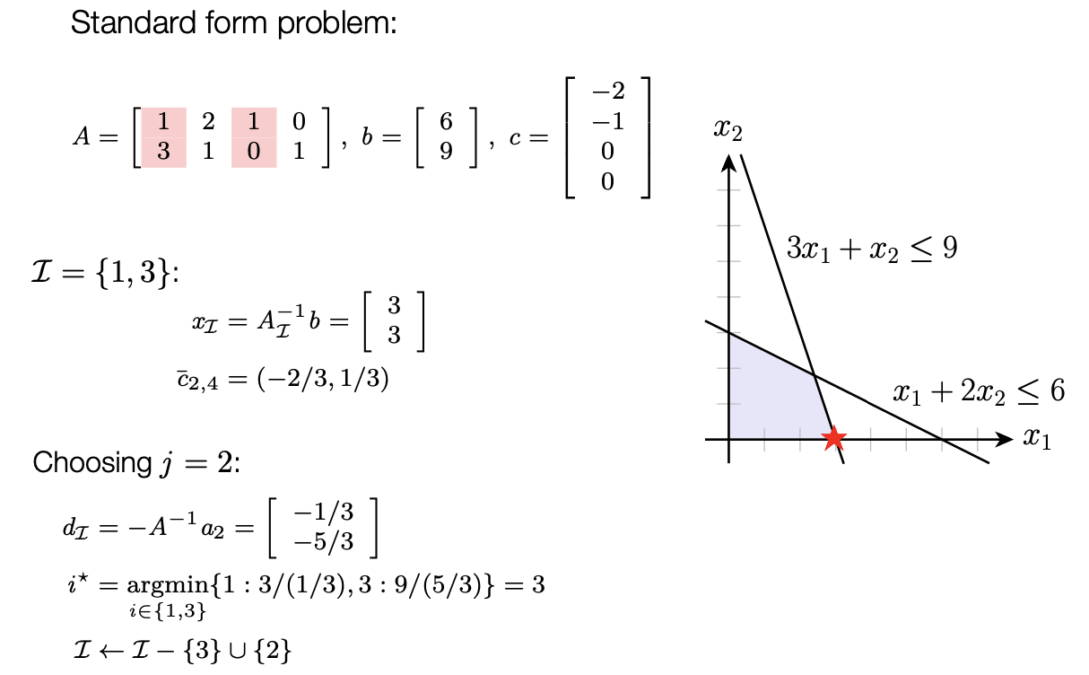
Illustration of simplex-3
Numerical considerations
Note that the above algorithm is described in terms of exact math
When implemented in floating point arithmetic, we’ll often get entries like \(\bar{c}_j, d_i \in\left[-10^{-15}, 10^{-15}\right]\)
When comparing to zero, or comparing “ties” (especially under degeneracy, see next slide), we need to account for this
In practice, set these near-zero elements to zero or compare \(\geq, \leq\) to \(\pm 10^{-12}\)
Degeneracy
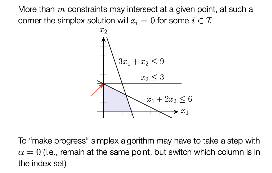
Handling degeneracy
Simplex will still work fine with zero step sizes, but care must be taken to prevent cycling repeatedly over the same indices
A similar issue can occur when determining which \(i^{\star}\) exits the index set (more than one \(x_i\) becomes zero at the same time)
A simple approach to fix these issues, Bland’s rule: 1. At each step, choose smallest \(j\) such that \(\bar{c}_j<0\) 2. From variables \(x_i\) that could exit index set, choose smallest \(i\)
Alternatively, perturb \(b\) by some small noise and then solve
Finding feasible solutions
We assumed a feasible initial point (i.e. \(\mathcal{I}\) such that \(A_{\mathcal{I}} b \geq 0\) )
To find such a point (in cases where it is not easy to construct one), we introduce variables \(y \in \mathbb{R}^m\) and solve auxiliary problem \[ \begin{aligned} \underset{x, y}{\operatorname{minimize}} & 1^T y \\ \text { subject to } & A x+y=b \\ & x, y \geq 0 \end{aligned} \]
A standard form linear program, with feasible solution \(x=0, y=b\), (if \(b_i<0\), replace constraint \(a_i^T x=b_i\) with \(-a_i^T x=-b_i\) )
If solution to this problem has \(y=0\), we know \(A x=b\), so we have found a feasible solution to the original problem (though need to handle possible degeneracy)
Revised simplex
Simplex algorithm requires inverting \(A_{\mathcal{I}}\) at each iteration: naive implementation would re-invert this matrix every time \(\Longrightarrow O\left(m^3\right)\) computation at each iteration
Revised simplex algorithm directly maintains and updates this inverse \(\mathcal{A}_I^{-1}\) at each iteration, using \(O\left(m^2\right)\) computation
Key idea is the Sherman-Morrison inversion formula, for an invertible matrix \(C \in \mathbb{R}^{n \times n}\) and vectors \(u, v \in \mathbb{R}^n\) \[ \left(C+u v^T\right)^{-1}=C^{-1}-\frac{C^{-1} u v^T C^{-1}}{1+v^T C^{-1} u} \]
Suppose we update \(\mathcal{I}\) by dropping index \(\mathcal{I}_k\) and adding index \(j\)
Numerically, this is done by overwriting the column \(a_{\mathcal{I}_k}\) in \(A_{\mathcal{I}}\) with \(a_j\) (suppose this occurs at index \(I_k\) ), i.e., \[ A_{\mathcal{I}} \leftarrow A_{\mathcal{I}}+\left(a_j-a_{\mathcal{I}_k}\right) e_k^T \] where \(e_k\) is the \(k\) th basis vector (all zeros except for 1 at element \(k\) )
Using the Sherman-Morrison formula \[ \left(A_{\mathcal{I}}+\left(a_j-a_{\mathcal{I}_k}\right) e_k^T\right)^{-1}=A_{\mathcal{I}}^{-1}-\frac{A_{\mathcal{I}}^{-1}\left(a_j-a_{\mathcal{I}_k}\right) e_k^T A_{\mathcal{I}}^{-1}}{1+e_k^T A_{\mathcal{I}}^{-1}\left(a_j-a_{\mathcal{I}_k}\right)} \]
Right most expression can be written as an outer product matrix \(u v^T\), so forming and adding it to \(A_{\mathcal{I}}^{-1}\) takes \(O\left(m^2\right)\) operations
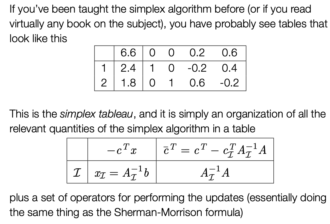
Simplex tableau
Source(s)
- 15-780: Linear Programming, J. Zico Kolter, https://www.cs.cmu.edu/afs/cs/academic/class/15780-s16/www/slides/linear_prog.pdf
Appendix
Review: Matrix math
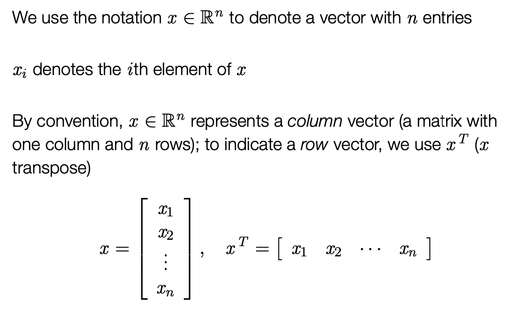
Vectors
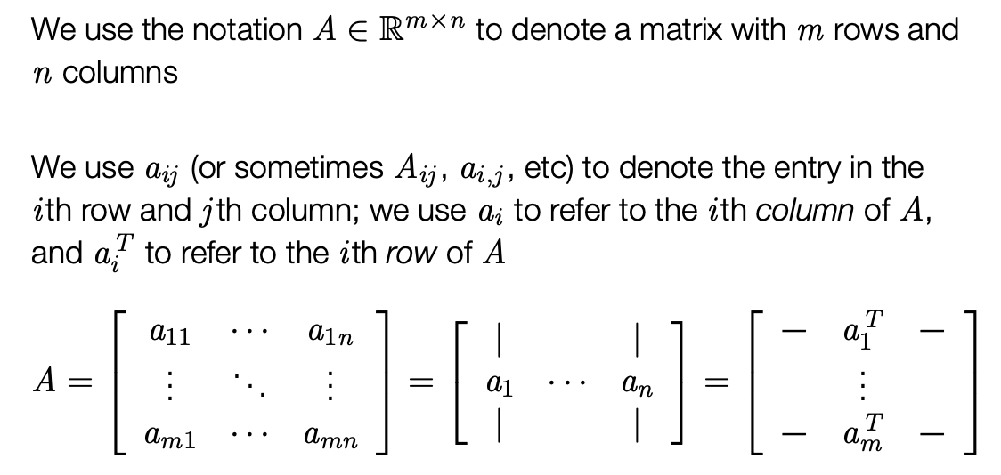
Matrices
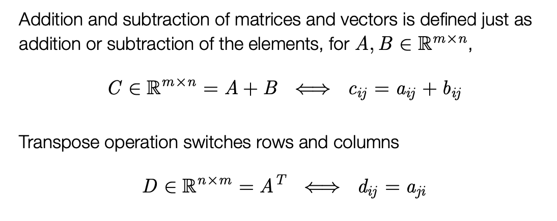
Addition/subtraction and transposes
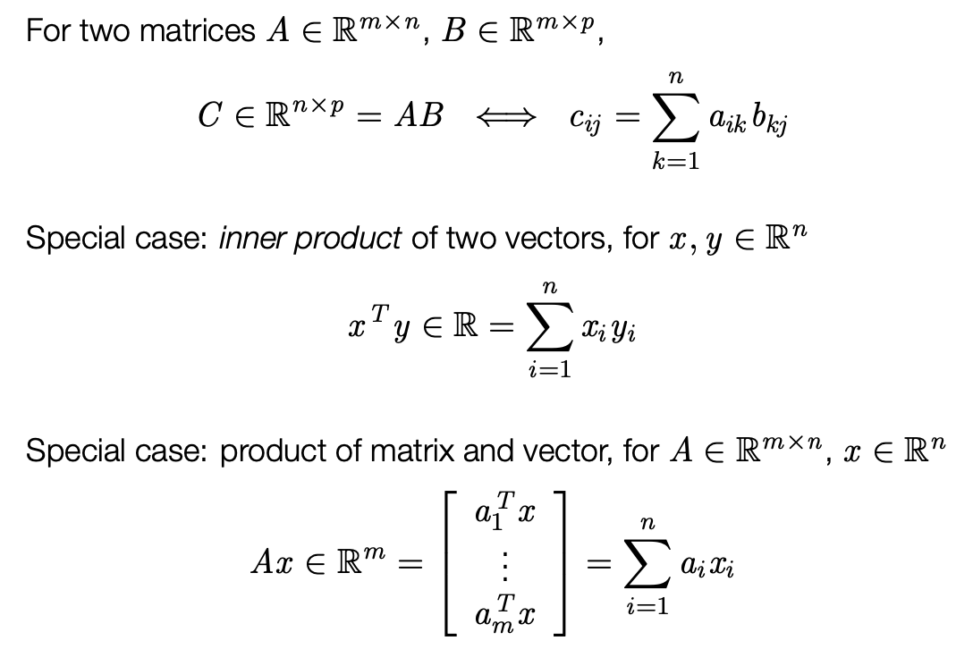
Matrix multiplication
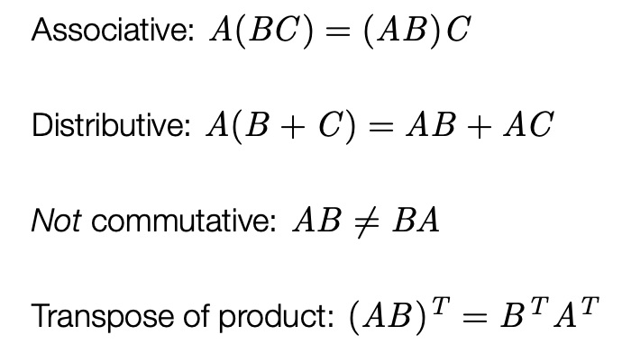
Matrix multiplication properties
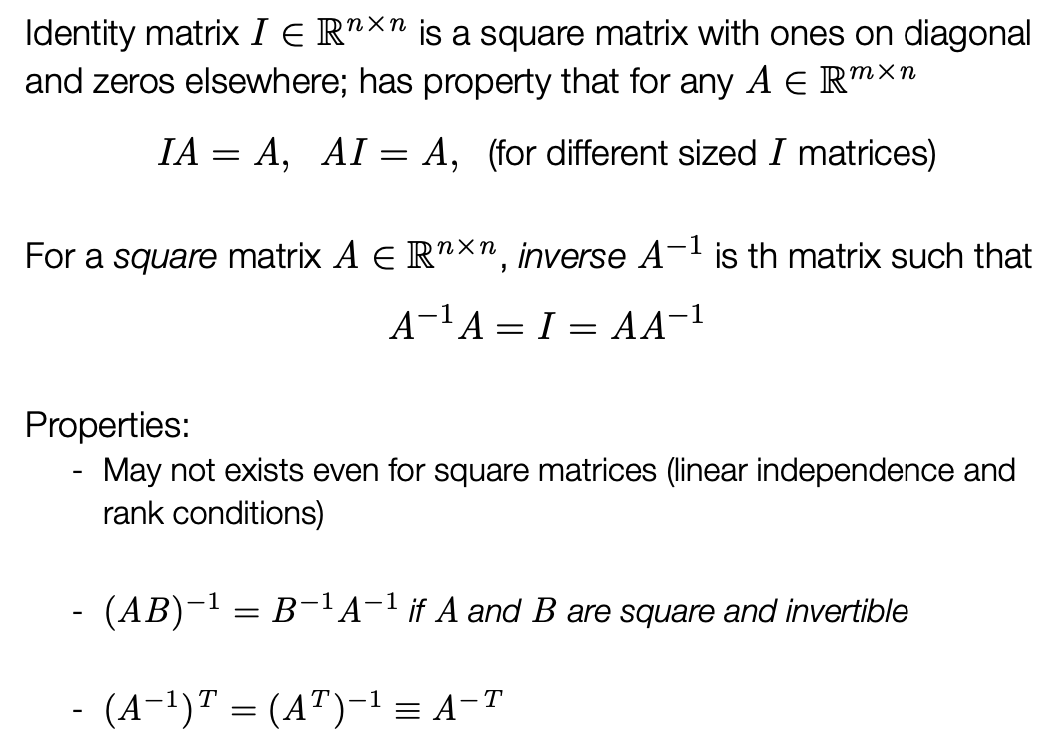
Matrix inverse
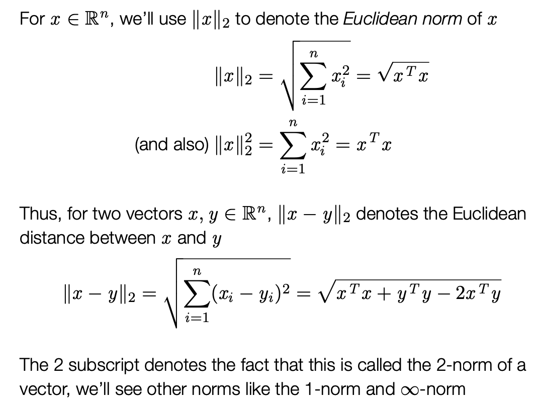
Vector norms