Dynamic network models
Overview of common dynamic network models
Recording
The following is a recording on this topic, I hope you find it useful!
Feel free to watch at 1.5x or 2x speed.
Note: If you find something missing or incorrect in the recording, then please let me know!
Epidemic and Meme diffusion
Introduction
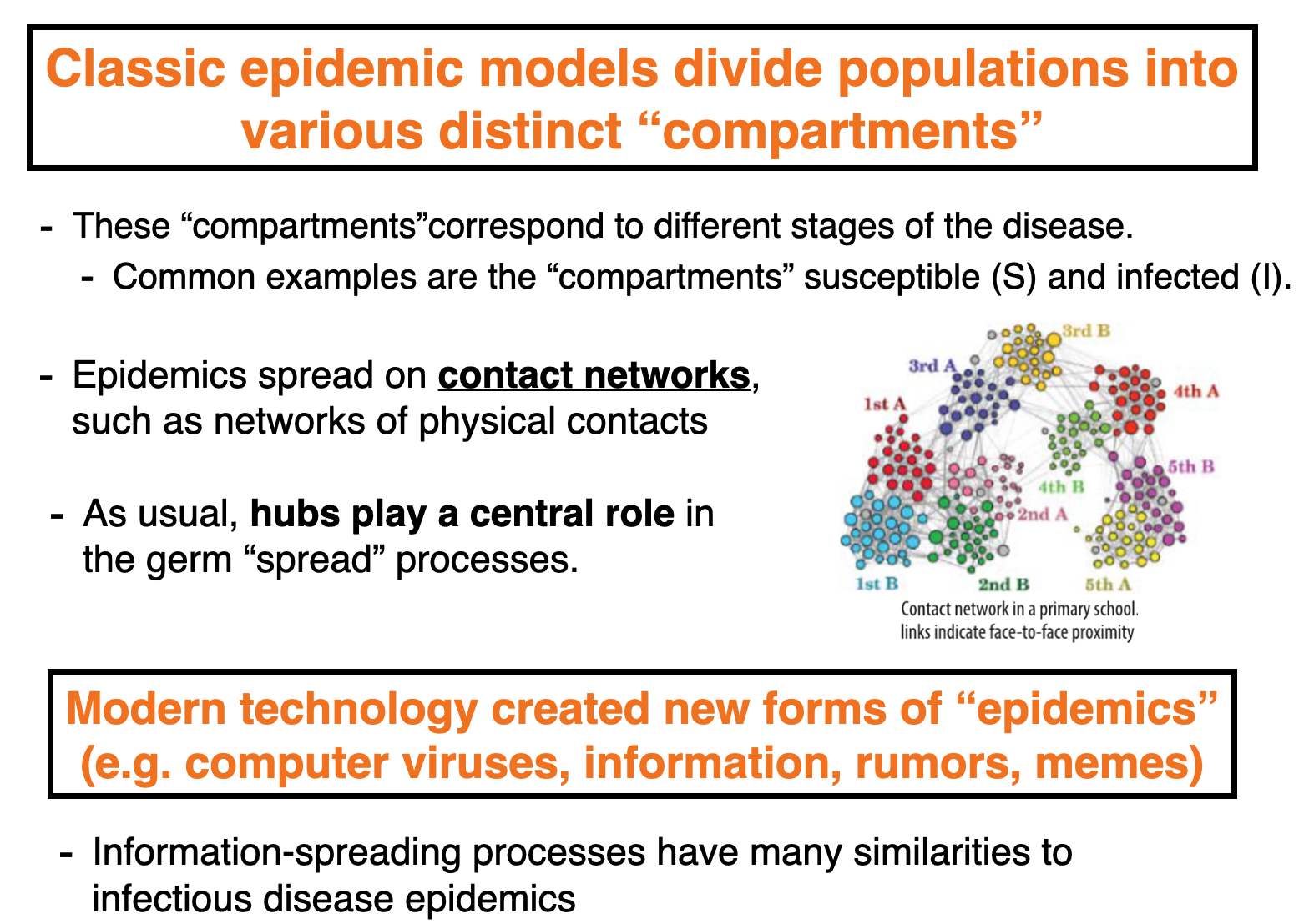
Model-4: (SIS) model
- Susceptible-infected-susceptible (SIS) model
- Infected individuals become susceptible again after recovery
- Applies to diseases without long-lasting immunity (e.g. common cold)
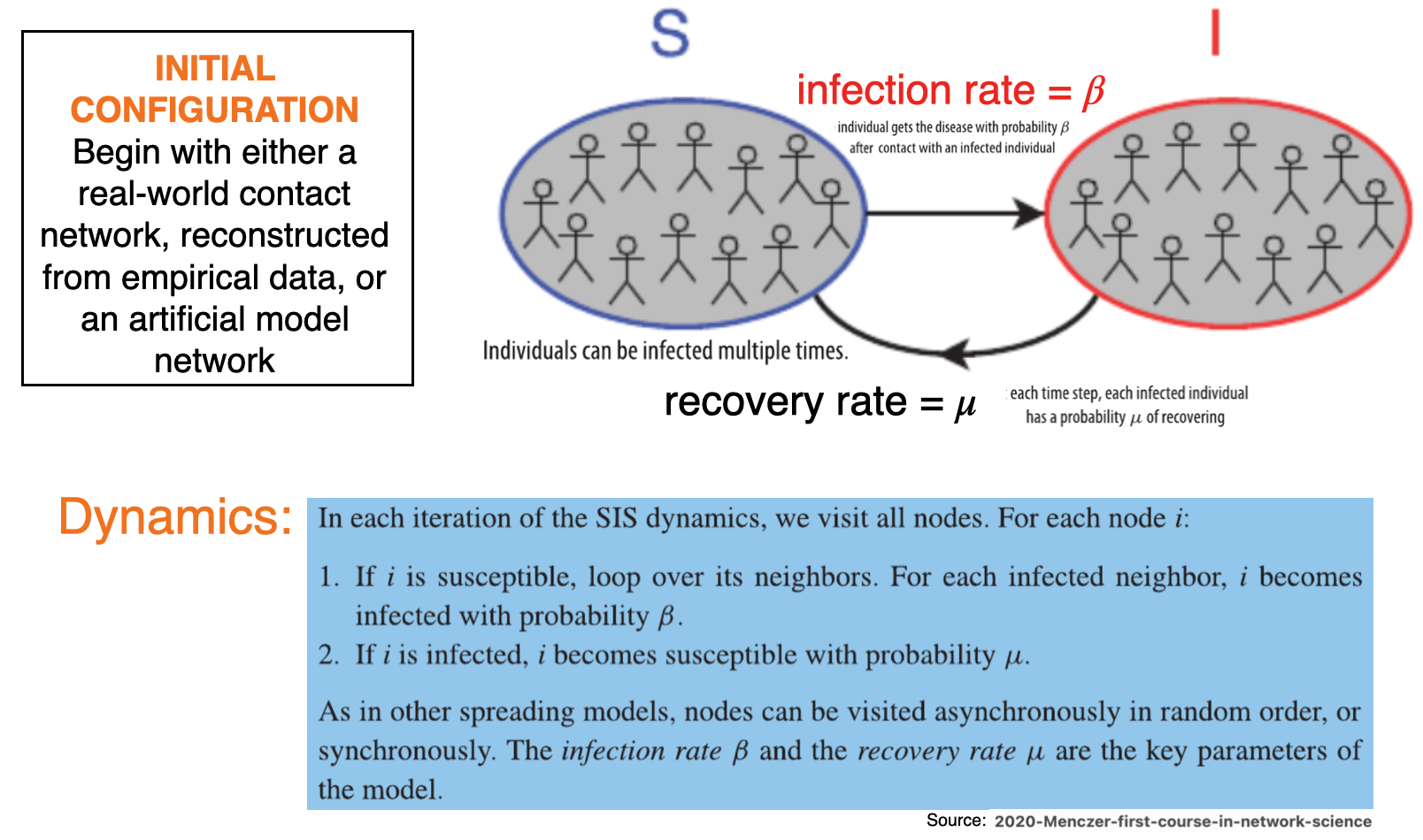
Example
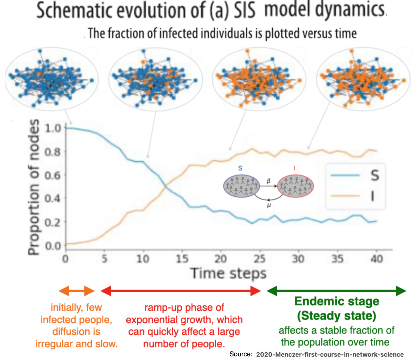
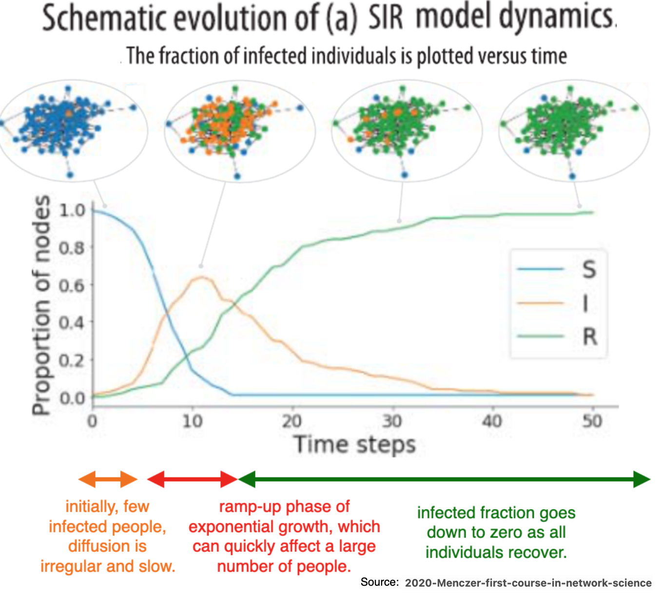
Model-5: Susceptible-infected-recovered (SIR) model.
- Infected individuals recover, and move to a third compartment, recovered (R), where individuals cannot be infected anymore
- Applies to diseases WITH long-lasting immunity (e.g. measles, mumps, rubella)
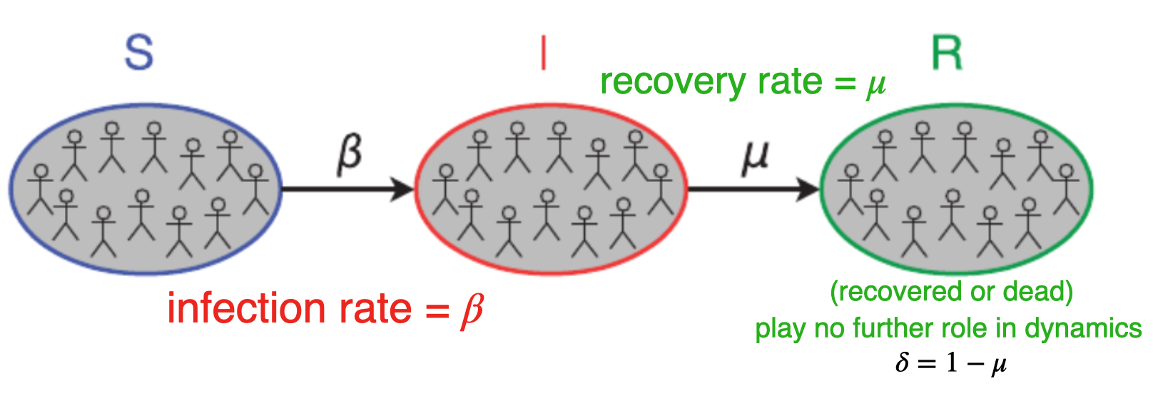
- The dynamics of infection and recovery follow closely those of the SIS model
- Eventually, the SIR model spreading stops, when there are no more infected individuals.
Example: SIR model
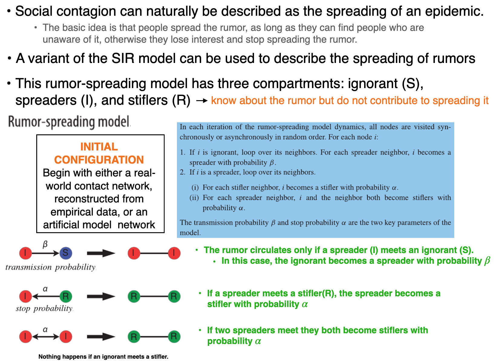
Rumor Spreading
Opinion dynamic models
Opinion:A view formed about something, not necessarily based on factOpinion dynamics: Processes that determine how opinions diffuse in society
Importance of opinions
- Opinions have important real-world implications, for example, they drive our behaviors, affect life choices, influence plans, and dictate purchase decisions.
- Policies implemented by governments worldwide are dictated by opinions about trade, conflicts, immigration, pandemics, the environment, and so on.
- We can represent opinions numerically as a number or a set of numbers.
Model overview
Opinion models are usually divided into two categoriesDiscrete opinions(integer values) -When there are a limited discrete number of positions on a specific issue- The opinion can be represented by an integer attribute (state) of each node.
- Examples: buy/sell, left/right, voting, like or dislike, Android/iPhone/flip-phone
Continuous opinions(real-valued)- Situations where opinion can vary smoothly from one extreme to the other in a range of possible choices.
- Examples: impression` of art or music, political alignment,
Possible outcomes
- Possible outcomes
- System reaches a steady state (i.e. node opinions don’t change anymore)
consensus:all nodes having the same opinion,polarization:some nodes holding an opinion and the rest holding the other
- The system does not reach a stationary state
- Some nodes (or all) keep changing their opinions at each iteration.
- However, some features of the opinion configuration, for example the averages of some variables, may stabilize in the long run.
Structure-dynamic relation- In most situations there is an interplay between network structure and it’s dynamics
- i.e. structure effects dynamics and dynamics in turn changes the network structure
Binary opinion models
- For simplicity, consider the special case of binary opinions (voting, buy/sell, yes/no)
- As before, a model is characterized by the set of rules that determine how the opinion of a node changes due to the opinions of its neighbors.
The model dynamics usually follow these steps:- Initial configuration: opinions are randomly assigned among the nodes
- approximately same number of people holding either opinion (disagreement)
- Dynamic rules: Update rule is applied over and over to all nodes.
- An iteration consists of running a loop over al nodes.
- Typically, nodes are updated asynchronously in a random order
Binary opinion variables
A few standard variables can be computed and monitored in these models:
Average opinion: The arithmetic average of the opinions across the nodes.- Random distribution of two opinions (0,1) \(\rightarrow\) the average is around 0.5
- The average opinion has a temporal dependence (i.e. changes during the dynamics)
- If the system reaches a stationary state, then the average converges to a precise value.
- If the stationary state is consensus, it equals either zero or one, depending on which opinion dominates.
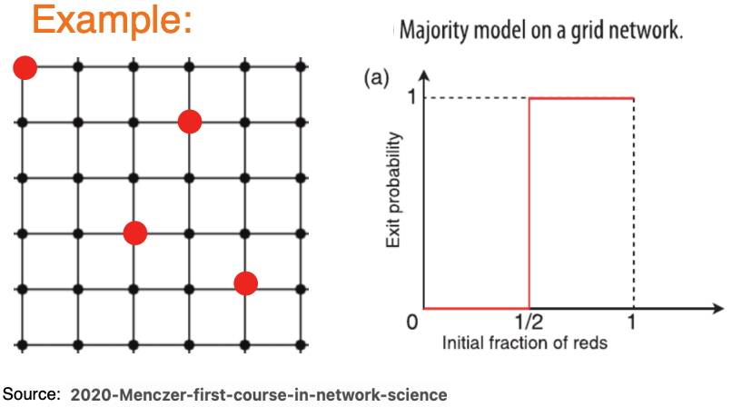
Exit probability: Probability that the network is to reach consensus to opinion one, as a function of the fraction of nodes with opinion one in the initial configuration.- As an illustration, suppose that we run the model dynamics 100 times, starting from 100 different random configurations.
- In each initial configuration we assign opinion one to every node with probability 0.4 , so that approximately \(40 \%\) of the nodes will have opinion one.
- Imagine that all runs lead to consensus (no polarization), 30 of them to consensus opinion one.
- The value of the exit probability for initial probability 0.4 of opinion one is then \(30 / 100=0.3\)
Majority model
- The dynamics are based on a majority rule: i.e. each node takes the opinion of the majority of its neighbors
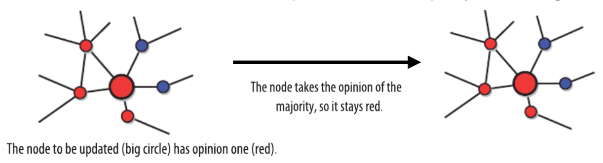
- Resolving ties: If the number of neighbors is even and there is an equal number with either opinion, then flip a coin to decide which opinion wins
Majority model: dynamic behavior
- In order to reach consensus on any opinion, that opinion must have the majority in the initial configuration.
Voter model
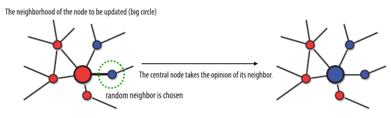
- Each node takes the opinion of a randomly chosen neighbor, whatever it may be.
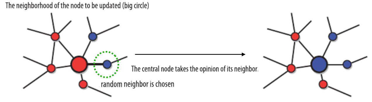
- Consensus is the only stable state of the voter model dynamics, so it is the inevitable final configuration of the system
Voter model: dynamic behavior
- The outcome of the dynamics is uncertain
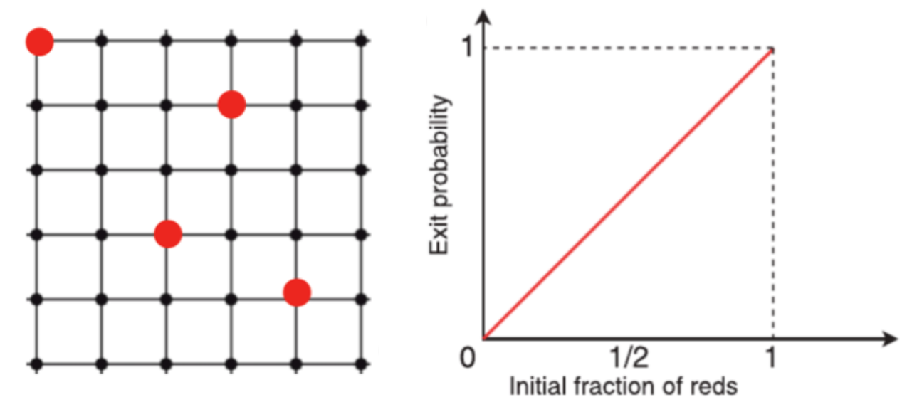
- The exit probability of the voter model coincides with the fraction of initial nodes with opinion one.
- The diagonal function indicates that the initial proportion of opinions one is also the probability of reaching consensus on opinion one.
Variants of the voter model
- The presence of zealots, nodes who never change their opinion. If they all have the same opinion, they will favor consensus around that opinion, otherwise consensus is never reached.
- Considering more than two opinion states. In this case, the interactions may be constrained to occur only among nodes with sufficiently close opinions. For example one could have three opinions \((1,2\), and 3 ) such that only neighboring opinions can interact (1 and 2, 2 and 3, but not 1 and 3). We discuss such a principle in detail in Section 7.3.2. Non-consensus configurations with non-interacting opinions are stable in any network.
- The possibility for nodes to change their opinion spontaneously, for example with a certain probability at each iteration, on top of the voter dynamics.
Coevolution of network structure and dynamics
- In the previous models, ONLY node attributes changed, NOT structure (inter-connectivity)
Structure-dynamic relation
- In most situations there is an interplay between network structure and it’s dynamics
- i.e. structure effects dynamics and dynamics in turn changes the network structure
- Recall that
assortativityis found in many real graphs, particularly social networks- Degree assortativity is the tendency of similar degree nodes to bond together (birds of a feather flock together)
- social influence (neighbors becoming more similar)
- homophily (aka selection) (similar nodes becoming neighbors)
Coevolution models:
- Models where opinion changes may induce modifications in the network structure, which could in turn affect the opinions, and so on.
- Basically, opinions and networks adapt and respond to each other.
Coevolution of network structure and dynamics
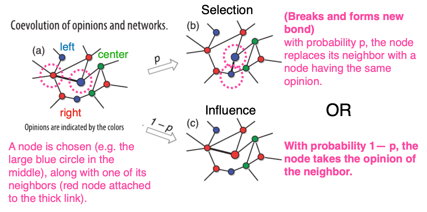
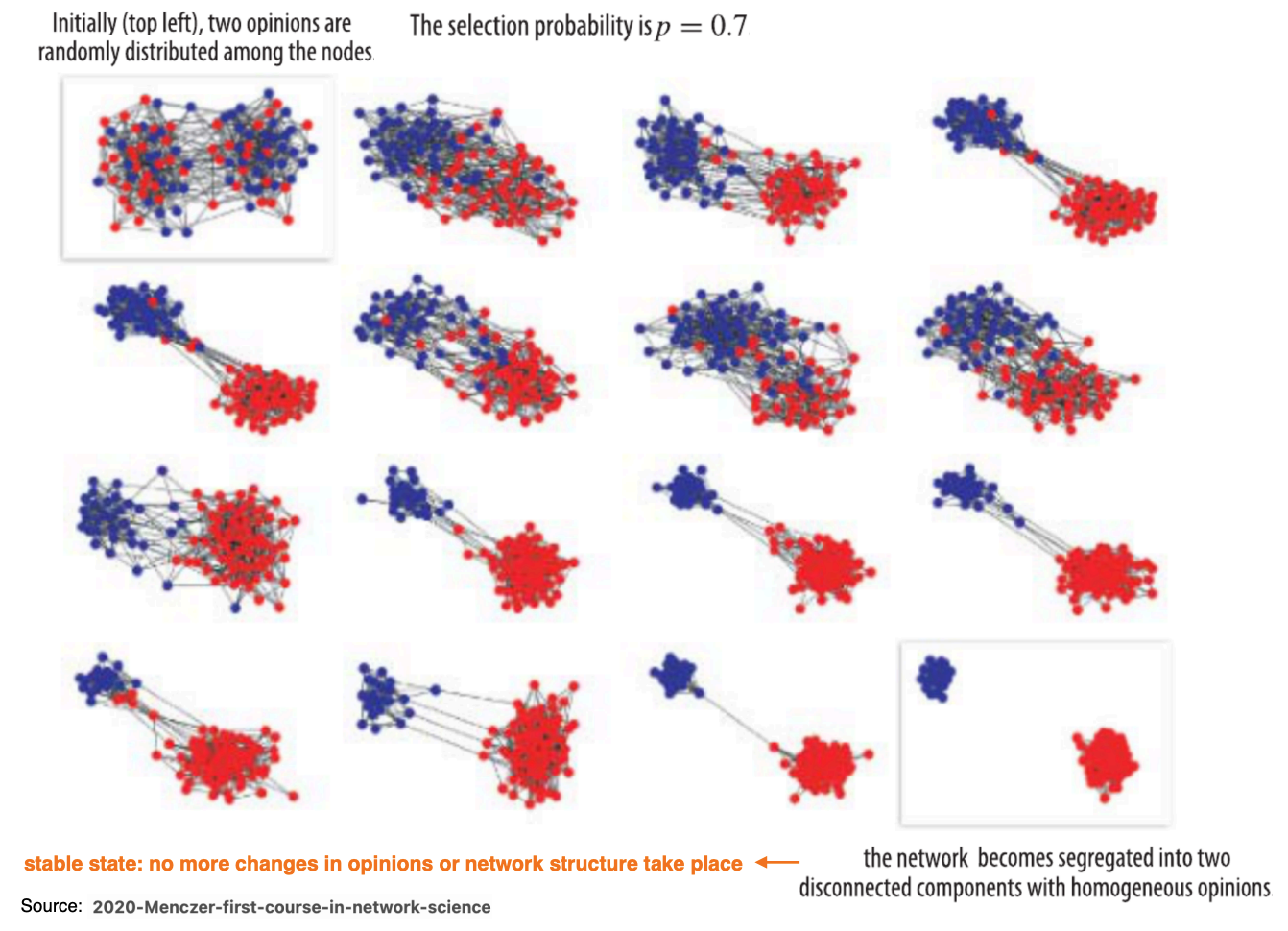
- At the beginning, opinions are randomly assigned to the nodes.
Algorithm
- Each iteration of the coevolution model requires a sweep over the nodes, synchronously or in random order. When we examine node \(i\), we select a random neighbor \(j\) with different opinion from \(i\) :
- With probability \(p\), the link between \(i\) and \(j\) is rewired from \(i\) to a randomly selected non-neighbor holding the same opinion as \(i\) (selection).
- Else (with probability \(1-p\) ), \(i\) takes the opinion of \(j\) (influence).
- The selection probability \(p\) is the single parameter of the model.
Coevolution model dynamics
Bounded-confidence model (BCM)
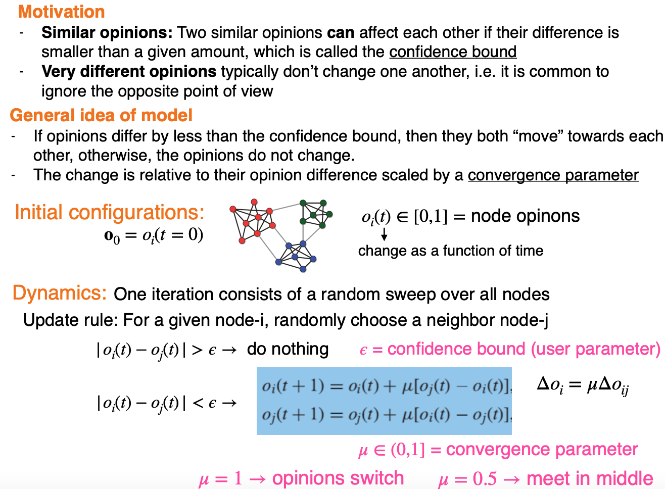
- The original bounded-confidence model has an update rule that consists of choosing a node and one of its neighbors.
- If their opinions differ by less than the confidence bound, they both “move” towards each other, by some relative amount determined by a convergence parameter.
- Otherwise, the opinions do not change.
Algorithm
In the bounded-confidence model, at iteration \(t\), each node \(i\) has opinion \(o_i(t)\), which is a real number between, say, zero and one. An iteration consists of a sweep over all nodes, synchronously or in random order. At iteration \(t+1\), when it comes to node \(i\), we pick one of its neighbors at random, say \(j\). If \[ \left|o_i(t)-o_j(t)\right|<\epsilon, \] where \(\epsilon\) is the confidence bound, the values of the opinions are updated to \[ \begin{aligned} & o_i(t+1)=o_i(t)+\mu\left[o_j(t)-o_i(t)\right], \\ & o_j(t+1)=o_j(t)+\mu\left[o_i(t)-o_j(t)\right], \end{aligned} \] where \(\mu>0\) is the convergence parameter. If \(\mu=1 / 2\), the opinions converge to their average, meaning that both individuals adopt a common intermediate position. If \(\mu=1\) the opinions switch, in that \(i\) adopts \(j\) ’s opinion and vice versa. Usually \(\mu\) varies in the range \((0,1 / 2]\).
Summary (BCM)
Social diffusion mechanisms