import torch
from torch_geometric.data import Data
from torch_geometric.transforms import RandomNodeSplit

# Create toy node features: 10 nodes, each with 16 features
x = torch.randn(10, 16)  # [num_nodes, num_features]
# Create toy node labels: 10 nodes, 3 classes (0, 1, 2)
y = torch.randint(0, 3, (10, )) # [num_nodes]Data splitting for graph data
Recording
The following is a recording on this topic, I hope you find it useful!
Feel free to watch at 1.5x or 2x speed.
Note: If you find something missing or incorrect in the recording, then please let me know!
Notes
Overview
- Just like in regular machine learning, dataset splitting is essential for training, validation, and testing in graph based machine learning.
- We do it to prevent overfitting and enable proper model evaluation and generalization.
- Common techniques in PyG (PyTorch Geometric):
RandomNodeSplitandRandomLinkSplit. - Custom (non-random) splits can also be created.
- How we do the split depends on the learning task as hand
Node-level data splitting
For node classification or node regression tasks
RandomNodeSplit command
RandomNodeSplit in PyG is used to randomly divide nodes into training, validation, and test sets.
Works with both PyG Data and HeteroData objects.
Key parametersforRandomNodeSplitnum_val,num_test: Number or ratio of validation/test edges.is_undirected: Treats graph as undirected to prevent edge leakage.key: Attribute name for ground-truth labels.split_labels: Store positive/negative labels separately.add_negative_train_samples: Whether to add negative samples for training.neg_sampling_ratio: Ratio of negative to positive edges.disjoint_train_ratio: Use disjoint edges for supervision.edge_types,rev_edge_types: Specify edge types for splitting in HeteroData.
Example: Toy data set
- Lets start by creating a toy data set.
# Define toy edges (undirected for visualization)
edge_index = torch.tensor([
    [0, 1, 2, 3, 4, 5, 6, 7, 8, 9, 0, 2, 4, 6],
    [1, 2, 3, 4, 5, 6, 7, 8, 9, 0, 2, 4, 6, 8]
], dtype=torch.long)

# Explore the data
print("type of x, y, edge_index: ", type(x), type(y), type(edge_index))
print(f"Node features: {x.shape}")
print(f"Node labels: {y.shape}")
print(f"Edge indices: {edge_index.shape}")
type of x, y, edge_index: <class 'torch.Tensor'> <class 'torch.Tensor'> <class 'torch.Tensor'>
Node features: torch.Size([10, 16])
Node labels: torch.Size([10])
Edge indices: torch.Size([2, 14])Convert to PyG Data object
- Recall that PyG Data objects are a collection of node features, edge indices, and other attributes aborbed into a single object.
- Each object represents a single graph which can be converted to a networkx graph via the
to_networkx()method. - Given the data stored as torch tensors, we can convert to a PyG graph via the constructor
Data()
# Create PyG Data object
data = Data(x=x, y=y, edge_index=edge_index)
print(type(data))
<class 'torch_geometric.data.data.Data'>
# store a copy as a networkx graph, including node features for visualization
from torch_geometric.utils import to_networkx
G = to_networkx(data,node_attrs=['x'])

# sanity check
print(type(G))
print(G)
print(G.nodes[0])
print(len(G.nodes[0]['x']))
<class 'networkx.classes.digraph.DiGraph'>
DiGraph with 10 nodes and 14 edges
{'x': [0.6310891509056091, -0.7558268904685974, -0.7550930976867676, -1.4795610904693604, 0.683599591255188, 0.6355504989624023, 0.01612548530101776, -1.405216097831726, -0.09604500234127045, -0.41555461287498474, -0.15596747398376465, 0.2083640694618225, -0.6308029294013977, 0.6687617301940918, -1.6608461141586304, -0.9684350490570068]}
16
# visualize graph with networkx showing the node labels
import networkx as nx
import matplotlib.pyplot as plt
nx.draw(G, with_labels=True, node_color=y, node_size=500, font_color='white')
plt.show()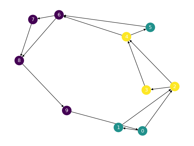
# Visualize based on average node features
print(x.mean(dim=0).shape,x.mean(dim=1).shape,x.shape)
nx.draw(G, with_labels=True, node_color=x.mean(dim=1), node_size=500, font_color='white')
torch.Size([16]) torch.Size([10]) torch.Size([10, 16])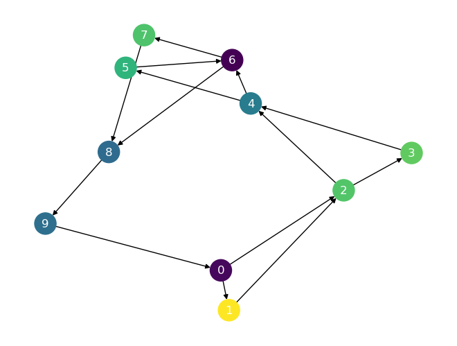
Split data into training, validation, and test sets
train_mask, valid_mask and test_mask will associated with each node
print(0.2*9,torch.floor(torch.tensor([0.2*9])))1.8 tensor([1.])# Randomly split nodes: 60-20-20 training,test,validation split
num_nodes=x.shape[0]
n_val=int(0.20*num_nodes)
n_test=int(0.20*num_nodes)
print(num_nodes,n_val,n_test)10 2 2# train=num_nodes-n_val-n_test
# for validation, 2 for test
node_transform = RandomNodeSplit(num_val=n_val, num_test=n_test)
node_splits = node_transform(data)
print(node_splits)Data(x=[10, 16], edge_index=[2, 14], y=[10], train_mask=[10], val_mask=[10], test_mask=[10])
# lets take a look at the masks
print(G.nodes)
print("Train:", node_splits.train_mask,torch.sum(node_splits.train_mask[node_splits.train_mask==True]))
print("Val:", node_splits.val_mask,torch.sum(node_splits.val_mask[node_splits.val_mask==True]))
print("Test:", node_splits.test_mask,torch.sum(node_splits.test_mask[node_splits.test_mask==True]))
[0, 1, 2, 3, 4, 5, 6, 7, 8, 9]
Train: tensor([ True, True, False, True, True, False, True, False, False, True]) tensor(6)
Val: tensor([False, False, True, False, False, True, False, False, False, False]) tensor(2)
Test: tensor([False, False, False, False, False, False, False, True, True, False]) tensor(2)Visualize the split
# Assign colors based on split masks
color_map = []
for i in range(data.num_nodes):
    if node_splits.train_mask[i]:
        color_map.append('tab:blue')      # Training nodes
    elif node_splits.val_mask[i]:
        color_map.append('tab:orange')    # Validation nodes
    elif node_splits.test_mask[i]:
        color_map.append('tab:green')     # Test nodes
    else:
        color_map.append('gray')          # Should not occur

plt.figure(figsize=(6, 4))
nx.draw(G, with_labels=True, node_color=color_map, node_size=500, font_color='white')
plt.title("Toy Graph with Train (blue)/Val (orange)/Test (green) Node Splits")
plt.show()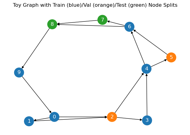
Edge-level data splitting
Overview
- RandomLinkSplit in PyG is used to randomly split edges into training, validation, and test sets
- Works with both Data and HeteroData objects
- num_val sets the number of validation edges
- num_test sets the number of test edges
- is_undirected specifies if the graph should be treated as undirected
Learning task: link prediction
Link predictionis a common learning task in graph machine learning where the goal is to predict whether an edge should exist between two nodes.- RandomLinkSplit is designed for binary classification of edges:
- Predict whether an edge exists (1) or does not exist (0).
- This is the standard link prediction task in most GNN pipelines.
- RandomLinkSplit is not intended for multi-class edge prediction out of the box. But you can handle multi-class edge tasks with custom logic:
Ran tool Ran tool The parameters of RandomLinkSplit are described in the markdown cells of your notebook. Here’s a summary based on the content in your file:
Parameters of RandomLinkSplit (PyTorch Geometric)
- num_val: Number (or ratio) of edges to use for the validation set.
- num_test: Number (or ratio) of edges to use for the test set.
- is_undirected: Boolean, specifies if the graph should be treated as undirected during splitting.
- key: The attribute name for ground-truth edge labels (e.g.,
'edge_y'). - add_negative_train_samples: Whether to add negative samples for training (default is
True). - neg_sampling_ratio: Ratio of negative to positive edges for negative sampling.
- disjoint_train_ratio: Use disjoint edges for supervision (for link prediction tasks).
- edge_types: (For HeteroData) Specify which edge types to split.
- rev_edge_types: (For HeteroData) Specify reverse edge types for splitting.
Summary Table
| Parameter | Description |
|---|---|
| num_val | Number or ratio of validation edges |
| num_test | Number or ratio of test edges |
| is_undirected | Treat graph as undirected for splitting |
| key | Attribute name for edge labels |
| add_negative_train_samples | Whether to add negative samples for training |
| neg_sampling_ratio | Ratio of negative to positive edges |
| disjoint_train_ratio | Use disjoint edges for supervision |
| edge_types | (HeteroData) Edge types to split |
| rev_edge_types | (HeteroData) Reverse edge types for splitting |
Note: Negative edges
Negative Edge Sampling: For each split (train/val/test), it randomly samples non-existent edges as negative examples, matching the number of positive edges unless otherwise specified.
Negative edges = node pairs not connected in the original graph.
Used in link prediction to teach the model what not to link.
RandomLinkSplit:`
- Splits edges into train/val/test sets.
- Randomly samples negative edges for each split.
- Matches number of negative edges to positive ones (configurable).
Output includes:
pos_edge_label_index(positive edges)neg_edge_label_index(negative edges)
Negative edges are sampled uniformly, excluding real edges.
neg_sampling_ratiocan control the number of negatives per positive.
Outputs
edge_index: Edges used for message passing to compute node embeddings.- Usually same for all splits.
edge_y_index: edges (real + fake) used for prediction.edge_y: ground truth labels for those edges.y: typically unused in link prediction; reserved for node labels.
Example
Using the same data as in the previous example, we can split the edges into training, validation, and test sets.
from torch_geometric.transforms import RandomLinkSplit

# apply the transform to the data
edge_transform = RandomLinkSplit(num_val=3, num_test=4, key='edge_y', add_negative_train_samples=False,neg_sampling_ratio=1,is_undirected=False)
train_data, val_data, test_data = edge_transform(data)

# Notice how instead of using masks the split instead results in separate Data objects
print(data)
print(data.edge_index)
print("--------training data--------")
print(train_data)
print(train_data.edge_index)
print(train_data.y)
print(train_data.edge_y)
print(train_data.edge_y_index)
print("--------validation data--------")
print(val_data)
print(val_data.edge_index)
print(val_data.y)
print(val_data.edge_y)
print(val_data.edge_y_index)
print("--------test data--------")
print(test_data)
print(test_data.edge_index)
print(test_data.y)
print(test_data.edge_y)
print(test_data.edge_y_index)
Data(x=[10, 16], edge_index=[2, 14], y=[10])
tensor([[0, 1, 2, 3, 4, 5, 6, 7, 8, 9, 0, 2, 4, 6],
[1, 2, 3, 4, 5, 6, 7, 8, 9, 0, 2, 4, 6, 8]])
--------training data--------
Data(x=[10, 16], edge_index=[2, 7], y=[10], edge_y=[7], edge_y_index=[2, 7])
tensor([[4, 2, 3, 2, 7, 4, 0],
[5, 4, 4, 3, 8, 6, 1]])
tensor([1, 1, 2, 2, 2, 1, 0, 0, 0, 0])
tensor([1., 1., 1., 1., 1., 1., 1.])
tensor([[4, 2, 3, 2, 7, 4, 0],
[5, 4, 4, 3, 8, 6, 1]])
--------validation data--------
Data(x=[10, 16], edge_index=[2, 7], y=[10], edge_y=[6], edge_y_index=[2, 6])
tensor([[4, 2, 3, 2, 7, 4, 0],
[5, 4, 4, 3, 8, 6, 1]])
tensor([1, 1, 2, 2, 2, 1, 0, 0, 0, 0])
tensor([1., 1., 1., 0., 0., 0.])
tensor([[0, 6, 1, 1, 4, 6],
[2, 8, 2, 9, 8, 1]])
--------test data--------
Data(x=[10, 16], edge_index=[2, 10], y=[10], edge_y=[8], edge_y_index=[2, 8])
tensor([[4, 2, 3, 2, 7, 4, 0, 0, 6, 1],
[5, 4, 4, 3, 8, 6, 1, 2, 8, 2]])
tensor([1, 1, 2, 2, 2, 1, 0, 0, 0, 0])
tensor([1., 1., 1., 1., 0., 0., 0., 0.])
tensor([[9, 6, 5, 8, 5, 0, 4, 3],
[0, 7, 6, 9, 4, 9, 3, 9]])Example: Graph-level splits
- Graph datasets are often split into training, validation, and test sets.
- In graph prediction tasks, each graph is treated as an independent sample.
- Splitting is usually done according to a specified ratio.
- Some PyG datasets (e.g., PPI) already provide predefined splits for training, validation, and testing.
- A complete example using the PPI dataset can be found in examples/ppi.py.
from torch_geometric.datasets import PPI

path = './data/PPI'

# in this case the splits result in dataset objects rather than individual graphs
train_dataset = PPI(path, split='train')
val_dataset = PPI(path, split='val')
test_dataset = PPI(path, split='test')

# size of each dataset
print(len(train_dataset), len(val_dataset), len(test_dataset))

# explore the split
print(train_dataset[0])
print(val_dataset[0])
print(test_dataset[0])

# explore the first graph
print(train_dataset[0])
print(val_dataset[0])
print(test_dataset[0])
20 2 2
Data(x=[1767, 50], edge_index=[2, 32318], y=[1767, 121])
Data(x=[3230, 50], edge_index=[2, 97446], y=[3230, 121])
Data(x=[3224, 50], edge_index=[2, 100648], y=[3224, 121])
Data(x=[1767, 50], edge_index=[2, 32318], y=[1767, 121])
Data(x=[3230, 50], edge_index=[2, 97446], y=[3230, 121])
Data(x=[3224, 50], edge_index=[2, 100648], y=[3224, 121])
Custom Splits
- Custom node splits can be created if random splitting is not suitable for your use case.
- This is common in real world scenarios, such as large-scale heterogeneous graphs in e-commerce.
- Nodes may represent different entities like users, products, or merchants.
- Splits can be made based on specific criteria, such as separating new and old users to evaluate model performance on new users.
Sources
Source: Unless otherwise stated, content below is derived from the PyTorch Geometric official documentation https://pytorch-geometric.readthedocs.io/en/latest/tutorial