import networkx as nx
%matplotlib inlineCode Demonstation
Instructions
Read, run, and work through all tutorial content and do all exercises below
The labs generally consists of TWO parts (1) A lab-demonstration tutorial (2) A short lab-assignment (contained below)
Demonstration section: Typically, the instructor will work through this section during the lab period. It is meant to be educational, with various code examples provided for you. You should understand all code in the demonstration section and should run the cells on your local machine before attempting the assignment.
NOTE: It is recommended that you complete this .ipynb file in VS-code. Activate the anly645 environment by selecting the kernel in the upper-left corner of VS-code.
Submission:
- Export the completed assignment to HTML or PDF (preferably with Quarto) and upload it to Canvas.
- The final uploaded version should NOT have any code-errors present
- All outputs must be visible in the uploaded version, including code-cell outputs, images, graphs, etc
Chapter 2: Tutorial
Note that many exercises are followed by a block with some assert statements. These assertions may be preceded by some setup code. They are provided to give you feedback that you are on the right path – receiving an AssertionError probably means you’ve done something wrong.
Contents:
- Paths
- Connected components
- Directed paths & components
- Dataset: US air traffic network
1. Paths
Let’s start with a very simple, undirected network.
G = nx.Graph()

G.add_nodes_from([1,2,3,4])

G.add_edges_from([(1,2),(2,3),(1,3),(1,4)])

nx.draw(G, with_labels=True)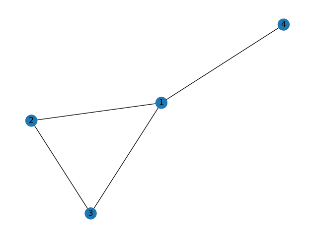
A path in a network is a sequence of edges connecting two nodes. In this simple example, we can easily see that there is indeed at least one path that connects nodes 3 and 4. We can verify this with NetworkX:
nx.has_path(G, 3, 4)TrueThere can be more than one path between two nodes. Again considering nodes 3 and 4, there are two such “simple” paths:
list(nx.all_simple_paths(G, 3, 4))[[3, 2, 1, 4], [3, 1, 4]]A simple path is one without any cycles. If we allowed cycles, there would be infinitely many paths because one could always just go around the cycle as many times as desired.
We are often most interested in shortest paths. In an unweighted network, the shortest path is the one with the fewest edges. We can see that of the two simple paths between nodes 3 and 4, one is shorter than the other. We can get this shortest path with a single NetworkX function:
nx.shortest_path(G, 3, 4)[3, 1, 4]If you only care about the path length, there’s a function for that too:
nx.shortest_path_length(G, 3, 4)2Note that a path length is defined here by the number of edges in the path, not the number of nodes, which implies
nx.shortest_path_length(G, u, v) == len(nx.shortest_path(G, u, v)) - 1for nodes \(u\) and \(v\).
2. Connected components
In the simple network above, we can see that for every pair of nodes, we can find a path connecting them. This is the definition of a connected graph. We can check this property for a given graph:
nx.is_connected(G)TrueNot every graph is connected:
G = nx.Graph()

# G.add_cycle((1,2,3))
G.add_edge(1,2)
G.add_edge(2,3)
G.add_edge(3,1)

G.add_edge(4,5)

nx.draw(G, with_labels=True)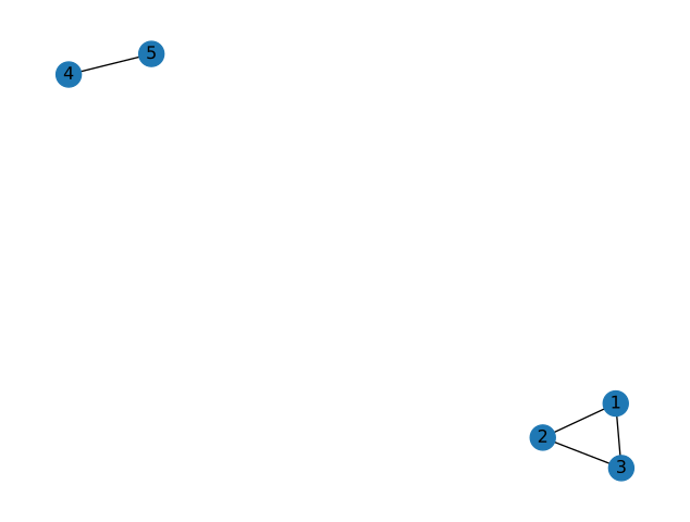
nx.is_connected(G)FalseAnd NetworkX will raise an error if you ask for a path between nodes where none exists:
nx.has_path(G, 3, 5)Falsenx.shortest_path(G, 3, 5)--------------------------------------------------------------------------- NetworkXNoPath Traceback (most recent call last) Cell In[11], line 1 ----> 1 nx.shortest_path(G, 3, 5) File ~/miniconda3/envs/anly503/lib/python3.10/site-packages/networkx/classes/backends.py:145, in _dispatch.<locals>.wrapper(*args, **kwds) 141 else: 142 raise NetworkXNotImplemented( 143 f"'{name}' not implemented by {plugin_name}" 144 ) --> 145 return func(*args, **kwds) File ~/miniconda3/envs/anly503/lib/python3.10/site-packages/networkx/algorithms/shortest_paths/generic.py:167, in shortest_path(G, source, target, weight, method) 164 else: 165 # Find shortest source-target path. 166 if method == "unweighted": --> 167 paths = nx.bidirectional_shortest_path(G, source, target) 168 elif method == "dijkstra": 169 _, paths = nx.bidirectional_dijkstra(G, source, target, weight) File ~/miniconda3/envs/anly503/lib/python3.10/site-packages/networkx/algorithms/shortest_paths/unweighted.py:224, in bidirectional_shortest_path(G, source, target) 221 raise nx.NodeNotFound(msg) 223 # call helper to do the real work --> 224 results = _bidirectional_pred_succ(G, source, target) 225 pred, succ, w = results 227 # build path from pred+w+succ File ~/miniconda3/envs/anly503/lib/python3.10/site-packages/networkx/algorithms/shortest_paths/unweighted.py:292, in _bidirectional_pred_succ(G, source, target) 289 if w in pred: # found path 290 return pred, succ, w --> 292 raise nx.NetworkXNoPath(f"No path between {source} and {target}.") NetworkXNoPath: No path between 3 and 5.
Visually, we can identify two connected components in our graph. Let’s verify this:
nx.number_connected_components(G)2The nx.connected_components() function takes a graph and returns a list of sets of node names, one such set for each connected component. Verify that the two sets in the following list correspond to the two connected components in the drawing of the graph above:
list(nx.connected_components(G))[{1, 2, 3}, {4, 5}]In case you’re not familiar with Python sets, they are collections of items without duplicates. These are useful for collecting node names because node names should be unique. As with other collections, we can get the number of items in a set with the len function:
components = list(nx.connected_components(G))
len(components[0])3We often care about the largest connected component, which is sometimes referred to as the core of the network. We can make use of Python’s builtin max function in order to obtain the largest connected component. By default, Python’s max function sorts things in lexicographic (i.e. alphabetical) order, which is not helpful here. We want the maximum connected component when sorted in order of their sizes, so we pass len as a key function:
max(nx.connected_components(G), key=len){1, 2, 3}While it’s often enough to just have the list of node names, sometimes we need the actual subgraph consisting of the largest connected component. One way to get this is to pass the list of node names to the G.subgraph() function:
core_nodes = max(nx.connected_components(G), key=len)
core = G.subgraph(core_nodes)

nx.draw(core, with_labels=True)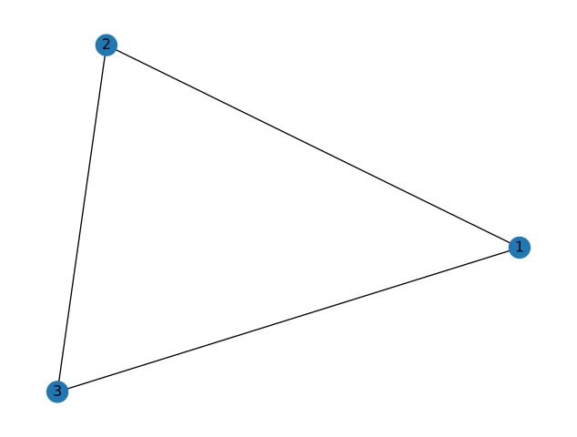
Those of you using tab-completion will also notice a nx.connected_component_subgraphs() function. This can also be used to get the core subgraph but the method shown is more efficient when you only care about the largest connected component.
3. Directed paths & components
Let’s extend these ideas about paths and connected components to directed graphs.
D = nx.DiGraph()
D.add_edges_from([
    (1,2),
    (2,3),
    (3,2), (3,4), (3,5),
    (4,2), (4,5), (4,6),
    (5,6),
    (6,4),
])
nx.draw(D, with_labels=True)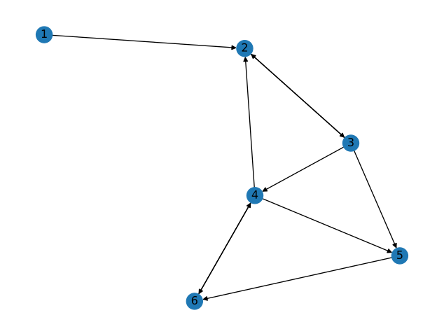
Directed paths
We know that in a directed graph, an edge from an arbitrary node \(u\) to an arbitrary node \(v\) does not imply that an edge exists from \(v\) to \(u\). Since paths must follow edge direction in directed graphs, the same asymmetry applies for paths. Observe that this graph has a path from 1 to 4, but not in the reverse direction.
nx.has_path(D, 1, 4)Truenx.has_path(D, 4, 1)FalseThe other NetworkX functions dealing with paths take this asymmetry into account as well:
nx.shortest_path(D, 2, 5)[2, 3, 5]nx.shortest_path(D, 5, 2)[5, 6, 4, 2]Since there is no edge from 5 to 3, the shortest path from 5 to 2 cannot simply backtrack the shortest path from 2 to 5 – it has to go a longer route through nodes 6 and 4.
Directed components
Directed networks have two kinds of connectivity. Strongly connected means that there exists a directed path between every pair of nodes, i.e., that from any node we can get to any other node while following edge directionality. Think of cars on a network of one-way streets: they can’t drive against the flow of traffic.
nx.is_strongly_connected(D)FalseWeakly connected means that there exist a path between every pair of nodes, regardless of direction. Think about pedestrians on a network of one-way streets: they walk on the sidewalks so they don’t care about the direction of traffic.
nx.is_weakly_connected(D)TrueIf a network is strongly connected, it is also weakly connected. The converse is not always true, as seen in this example.
The is_connected function for undirected graphs will raise an error when given a directed graph.
# This will raise an error
nx.is_connected(D)
--------------------------------------------------------------------------- NetworkXNotImplemented Traceback (most recent call last) Cell In[24], line 2 1 # This will raise an error ----> 2 nx.is_connected(D) File <class 'networkx.utils.decorators.argmap'> compilation 12:3, in argmap_is_connected_9(G) 1 import bz2 2 import collections ----> 3 import gzip 4 import inspect 5 import itertools File ~/miniconda3/envs/anly503/lib/python3.10/site-packages/networkx/utils/decorators.py:86, in not_implemented_for.<locals>._not_implemented_for(g) 82 def _not_implemented_for(g): 83 if (mval is None or mval == g.is_multigraph()) and ( 84 dval is None or dval == g.is_directed() 85 ): ---> 86 raise nx.NetworkXNotImplemented(errmsg) 88 return g NetworkXNotImplemented: not implemented for directed type
In the directed case, instead of nx.connected_components we now have nx.weakly_connected_components and nx.strongly_connected_components:
list(nx.weakly_connected_components(D))[{1, 2, 3, 4, 5, 6}]list(nx.strongly_connected_components(D))[{2, 3, 4, 5, 6}, {1}]4. Dataset: US air traffic network
This repository contains several example network datasets. Among these is a network of US air travel routes:
G = nx.read_graphml('openflights/openflights_usa.graphml.gz')
nx.draw(G)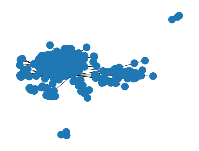
The nodes in this graph are airports, represented by their IATA codes; two nodes are connected with an edge if there is a scheduled flight directly connecting these two airports. We’ll assume this graph to be undirected since a flight in one direction usually means there is a return flight.
Thus this graph has edges
[('HOM', 'ANC'), ('BGM', 'PHL'), ('BGM', 'IAD'), ...]where ANC is Anchorage, IAD is Washington Dulles, etc.
These nodes also have attributes associated with them, containing additional information about the airports:
G.nodes['IND']{'name': 'Indianapolis International Airport',
'latitude': 39.7173,
'longitude': -86.294403,
'IATA': 'IND'}Node attributes are stored as a dictionary, so the values can be accessed individually as such:
G.nodes['IND']['name']'Indianapolis International Airport'Chapter 3: Tutorial
Contents:
1. Finding hubs
Often when looking at a network, we want to find the most “important” nodes, for some definition of important. The most basic measure of centrality is the degree, or number of links attached to a node.
Let’s look at the Enron executive email graph:
%matplotlib inline
import networkx as nx

G = nx.read_edgelist('ia-enron-only/ia-enron-only.edges', nodetype=int)
nx.draw(G)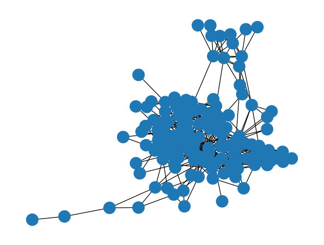
Caveat: by default, nx.read_edgelist assumes node names are strings
Edge lists are a simple, plain text format for storing graphs. Since this simple file format doesn’t contain information about data types, all node names are assumed to be strings by default. When the node names are given by integers, as they are in this example, we should specify the nodetype=int keyword argument to avoid confusion with the node names.
Aside: the max function
We’re going to make use of Python’s built-in max function in order to find the node with the highest degree.
First, let us recall what the max function does. At its most basic, the max function returns the “greatest” item in a sequence:
max([1,2,3,4,5])5But the “greatest” item is not always obvious:
max(['apple', 'grape', 'carrot'])'grape'Why is grape greater than the other options? Because the default sort for strings is lexicographical (basically alphabetical) order. If we don’t want this default ordering, we can specify a key function, which tells Python how to compare the items:
max(['apple', 'grape', 'carrot'], key=len)'carrot'Now carrot is the greatest element, because we’re comparing the items by their length.
Finding the node with max degree
We can apply the max function to get the maximum node according to some criterion. In our case, we want to compare the nodes by their degree:
highest_degree_node = max(G.nodes, key=G.degree)
highest_degree_node105G.degree(highest_degree_node)42So we know that node 105 has 42 edges connected to it. Let’s look at that calculation a little closer:
max(G.nodes, key=G.degree)We’re telling the max function that we want the item from G.nodes that gives us the highest value when passed to the key function G.degree.
This construction works because G.degree is a function. Some other measures of centrality such as betweenness generate all of the nodes’ centrality values at once and return a dict. In this case, we need an extra step:
betweenness = nx.centrality.betweenness_centrality(G)
highest_betweenness_node = max(G.nodes, key=betweenness.get)
highest_betweenness_node105betweenness[highest_betweenness_node]0.19400604344556296Note that the following will throw an error:
max(G.nodes, key=betweenness)--------------------------------------------------------------------------- TypeError Traceback (most recent call last) Cell In[42], line 1 ----> 1 max(G.nodes, key=betweenness) TypeError: 'dict' object is not callable
This is because we need to provide a function to the key argument, but betweenness is a dict. To get around this, we use the dict’s get method.
2. Centrality distributions
We’ve found the most central node in the network, but often we want to summarize information about the centrality of all nodes. For example, in addition to the maxmimum degree, we often want the mean and median degree in a network.
The first step in summarizing this information is to get a sequence of all of the centrality values in the graph. We don’t care about the node names anymore, we just want a sequence of numbers. We can start with the example of degree:
degree_sequence = [G.degree(n) for n in G.nodes]To get the mean and median of this sequence, we can use Python’s built-in statistics module:
import statistics

print('Mean degree:', statistics.mean(degree_sequence))
print('Median degree:', statistics.median(degree_sequence))
Mean degree: 8.713286713286713
Median degree: 8For other measures of centrality, which are calculated for the whole network at once and return a dict, we can use the dict’s .values().
betweenness = nx.centrality.betweenness_centrality(G)
betweenness_sequence = list(betweenness.values())

print('Mean betweenness:', statistics.mean(betweenness_sequence))
print('Median betweenness:', statistics.median(betweenness_sequence))
Mean betweenness: 0.013950388838012454
Median betweenness: 0.0037492834763570323Plotting the distribution
We can graphically represent the sequence of centrality values by using a histogram. In its basic form, a histogram plots the degree values on the x-axis, and the number of nodes having that degree on the y-axis. To do this counting, we can make use of Python’s collections.Counter.
from collections import Counter

degree_counts = Counter(degree_sequence)
degree_counts
Counter({30: 1,
2: 16,
17: 5,
12: 5,
13: 3,
16: 5,
10: 9,
11: 10,
18: 3,
20: 1,
15: 3,
19: 2,
7: 9,
14: 6,
9: 16,
42: 1,
8: 6,
5: 8,
6: 7,
1: 6,
4: 11,
23: 1,
3: 9})The Counter object returned is like a dict, pairing the item counted with the number of times it showed up in the sequence.
On this basic histogram plot, we want an x-value for every integer between the minimum and maximum degree in the sequence, inclusive. Note that degree_counts.keys() gives us every distinct value seen in the degree sequence. Also note that we need the +1 in the range below because we want to include the right endpoint.
min_degree, max_degree = min(degree_counts.keys()), max(degree_counts.keys())

plot_x = list(range(min_degree, max_degree + 1))
Our y-values are then the number of times we counted each x-value in the degree sequence. We can make use of the .get method with a default value in order to count 0 for degree values that don’t show up in the sequence. For example, notice that 32 does not show up in degree_counts above, so degree_counts.get(32, 0) will give us 0.
plot_y = [degree_counts.get(x, 0) for x in plot_x]To do the plotting, we use Matplotlib’s pyplot module.
import matplotlib.pyplot as plt

plt.bar(plot_x, plot_y)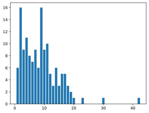
Histogram binning
When there are more x-values than you can comfortably display, or when your centrality measure is not discrete, as in the case of betweenness centrality, we can make use of histogram “binning.” This just defines a sequence of disjoint intervals called bins, and counts the number of values that fall into each such bin. In the simplest of cases, we can just tell Pyplot’s hist function how many bins we want and it will do the binning for us.
counts, bins, patches = plt.hist(betweenness_sequence, bins=10)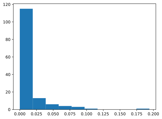
We can investigate the returned bins and counts if we want:
binsarray([0. , 0.0194006 , 0.03880121, 0.05820181, 0.07760242,
0.09700302, 0.11640363, 0.13580423, 0.15520483, 0.17460544,
0.19400604])countsarray([115., 13., 6., 4., 3., 1., 0., 0., 0., 1.])From these, we can see that there are 115 values between 0 and 0.0194006, 13 values between 0.194006 and 0.3880121, etc.