Statistical network analysis

Motivation

  • As we have seen, networks can be quantified mathematically using
    • scalars: typically for network-level quantities (e.g. average shortest path),
    • vectors: typically for node-level quantities (N) (e.g. node degree)
    • matrices: typically for edge (neighbor) level quantities \(N^2\) (e.g. adjacency matrix)
  • In general: To investigate the network, we can run statistical analysis on these quantities, e.g. summary stats, distributions, etc.
  • To better understand how centrality is distributed among the many nodes in large networks, we typically use a statistical approach.

Example: Degree distribution

  • The shape and range of the distribution reveals heterogeneity in the network
    • For example, if node degrees span many orders of magnitude, from units to millions, then the network is very heterogeneous

Source: Menczer1

Math review

Optional

Histograms

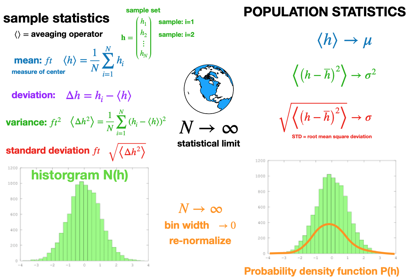
  • A histogram uses bars to display the frequency distribution of a dataset.

Statistical limit

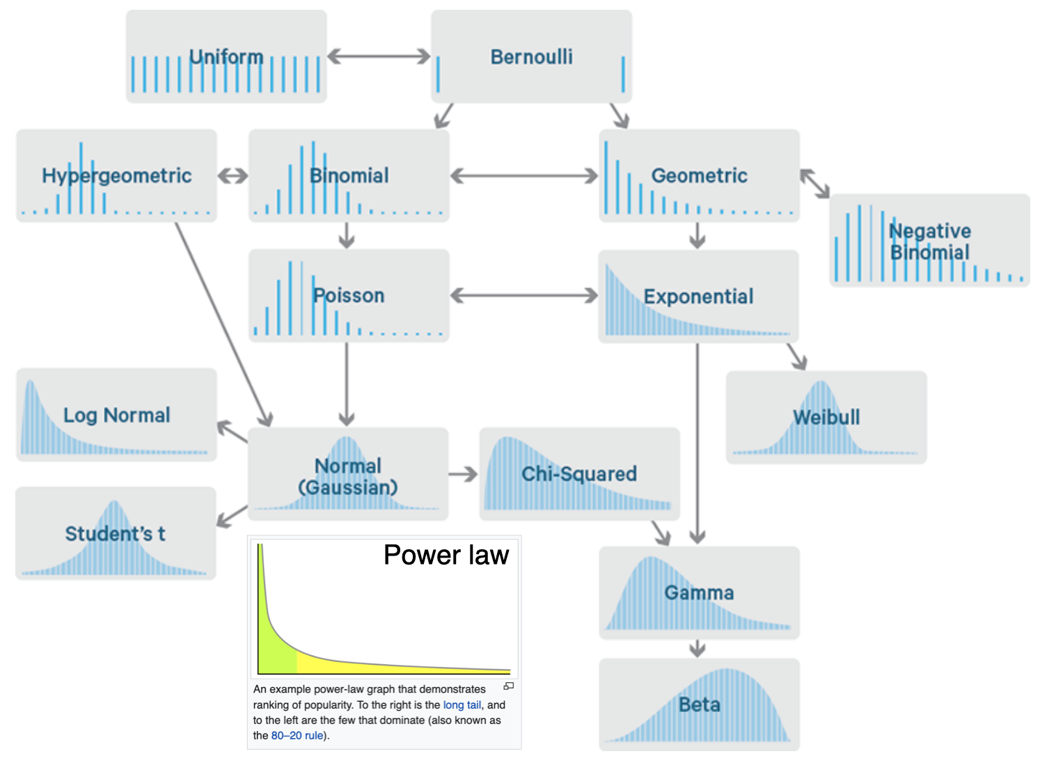
Common probability distributions

Numerical distribution types

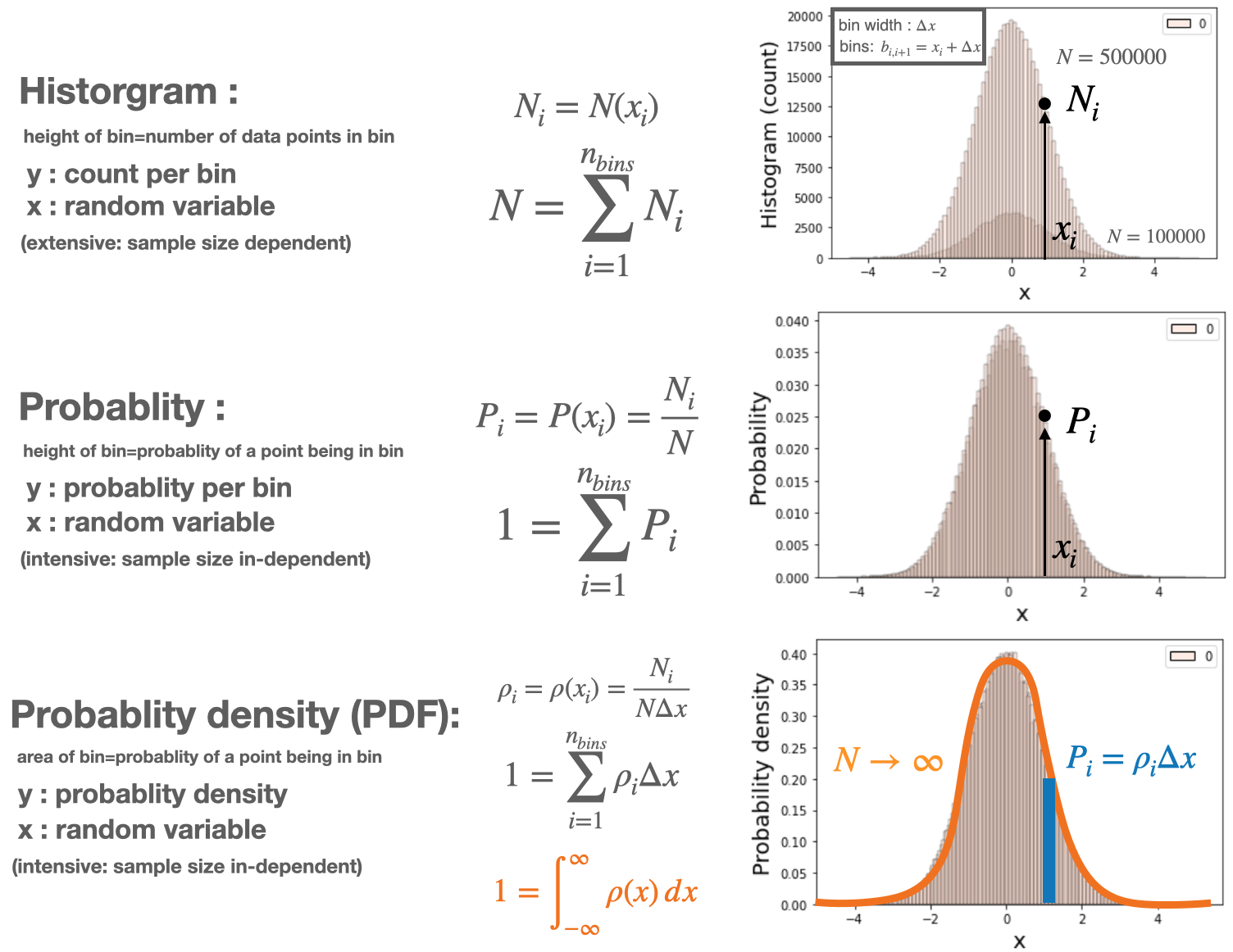
  • The following distributions all have similar functional forms, however, how we normalize changes the meaning of the quantity represented on the y-axis

Example: Numerical distributions

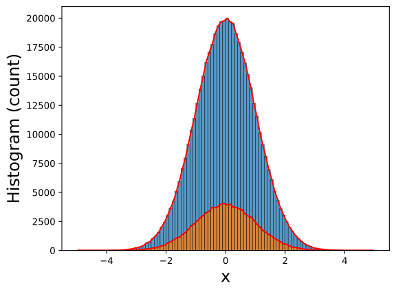
In the following we demonstrate the previous concept numerically for two sample sizes, consider a normal distribution

\[ f(x)=\frac{1}{\sigma \sqrt{2 \pi}} e^{-\frac{1}{2}\left(\frac{x-\mu}{\sigma}\right)^2} \]

# IMPORT
import matplotlib.pyplot as plt
import numpy as np
import seaborn as sns

# PARAM
BINS=100
FS=18
u=0.0
s=1.0
N1=100000
N2=5*N1 

# GENERATE SAMPLE DATA
x1=np.random.normal(u, s, size=(N1-2,1)); x1=np.append(x1,[u-5*s,u+5*s])
x2=np.random.normal(u, s, size=(N2-2,1)); x2=np.append(x2,[u-5*s,u+5*s])
# print(np.min(x1),np.max(x1))
# print(np.min(x2),np.max(x2))

# LINESPACE FOR PLOTTING
x3=np.linspace(np.min(x1),np.max(x1),100)

# DIRECT CALCULATE
(H1,B1)=np.histogram(x1,bins=BINS); 
B1=(B1[0:-1]+B1[1:])/2.0; dB1=B1[1]-B1[0] # midpoints
(H2,B2)=np.histogram(x2,bins=BINS)
B2=(B2[0:-1]+B2[1:])/2.0; dB2=B2[1]-B2[0] # midpoints
# print(dB1, dB2)

# # HISTOGRAM DISTRIBUTION
fig, ax = plt.subplots() # or what ever layout you want
sns.histplot(x2,bins=BINS,stat="count", kde=False,ax=ax)
ax.plot(B2,H2,'r-')
sns.histplot(x1,bins=BINS,stat="count", kde=False,ax=ax)
ax.plot(B1,H1,'r-')
ax.set_xlabel("x",fontsize=FS)
ax.set_ylabel("Histogram (count)",fontsize=FS)
plt.show()

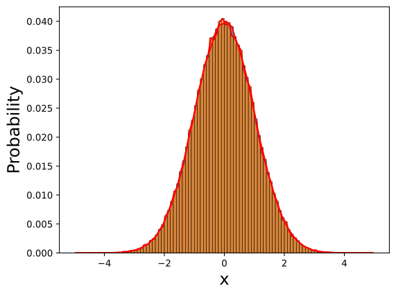
# # # PROBABILITY (LIKELIHOOD) DISTRIBUTION
fig, ax = plt.subplots() # or what ever layout you want
sns.histplot(x2,bins=BINS,stat="probability", kde=False,ax=ax)
ax.plot(B2,H2/N2,'r-')
sns.histplot(x1,bins=BINS,stat="probability", kde=False,ax=ax)
ax.plot(B1,H1/N1,'r-')
ax.set_xlabel("x",fontsize=FS)
ax.set_ylabel("Probability",fontsize=FS)
plt.show()

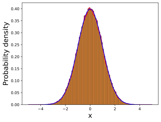
# # # PROBABILITY DENSITY DISTRIBUTION
fig, ax = plt.subplots() # or what ever layout you want
sns.histplot(x1,bins=BINS,stat="density", kde=False,ax=ax)
ax.plot(B2,H2/N2/dB2,'r-')
sns.histplot(x2,bins=BINS,stat="density", kde=False,ax=ax)
ax.plot(B1,H1/N1/dB1,'r-')
ax.set_xlabel("x",fontsize=FS)
ax.plot(x3,np.exp(-0.5*((x3-u)/s)**2.0)/(2.*np.pi*s)**0.5,'b-')
ax.set_ylabel("Probability density",fontsize=FS)
plt.show()

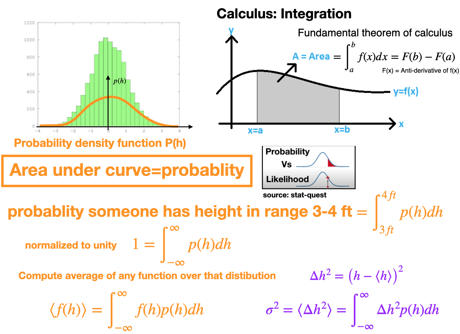
Probability density function

Cumulative distributions (CDF)

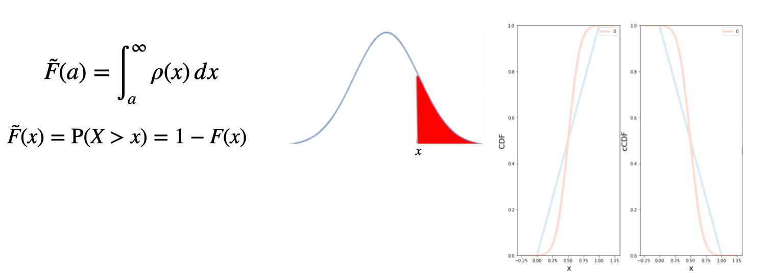
  • The Cumulative distribution function (CDF) of a continuous random variable \(X\) can be expressed as the integral of its probability density function \(f_X\) as \(F(a)=\int _{-\infty }^{a}\rho(x)\,dx\)

Complementary CDF: (cCDF)

  • Complementary cumulative distribution function (tail distribution)
  • Sometimes, it is useful to study the opposite question and ask how often the random variable is above a particular level.
  • This is called the complementary cumulative distribution function (ccdf) or simply the tail distribution or exceedance, and is defined as

Log-log plots

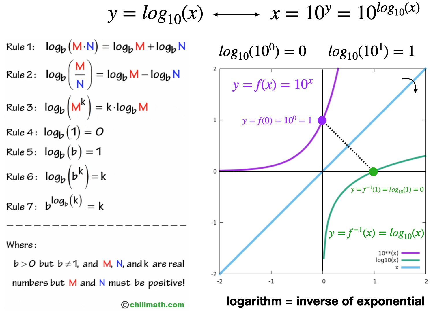
Recall: Logarithms

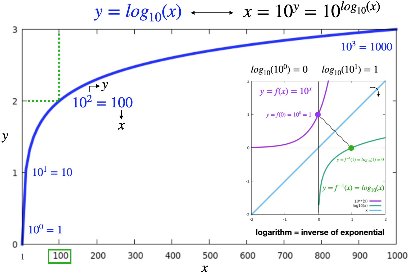
Recall: Logarithms

Log-scale

  • In network analysis, often we plot network quantities distributions on a log-log scale

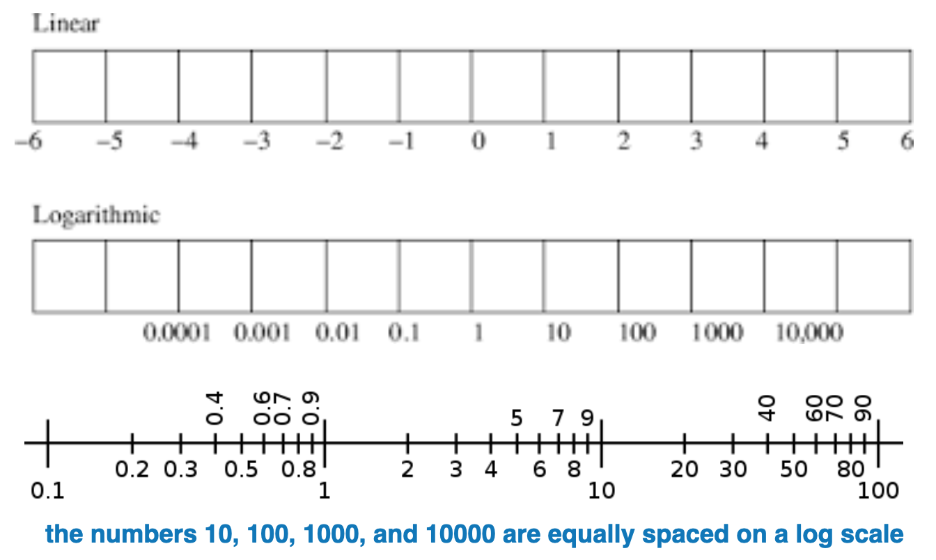
  • A logarithmic scale (or log scale) is a way of displaying numerical data over a very wide range of values in a compact way—typically the largest numbers in the data are hundreds or even thousands of times larger than the smallest numbers

  • Linear scale: Equal changes in data result in EQUAL differences in length encoding

  • Log-scale: Equal changes in data result in NON-EQUAL differences in length

source: https://en.wikipedia.org/wiki/Logarithmic_scale

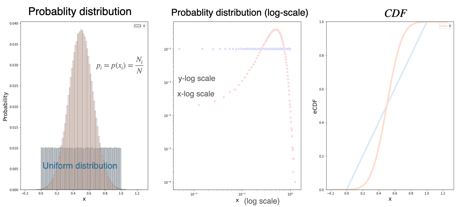
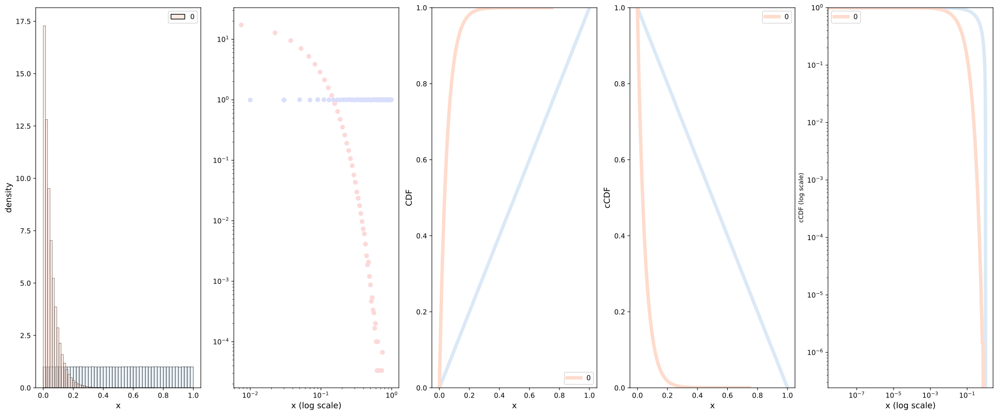
Example: Normal CDF

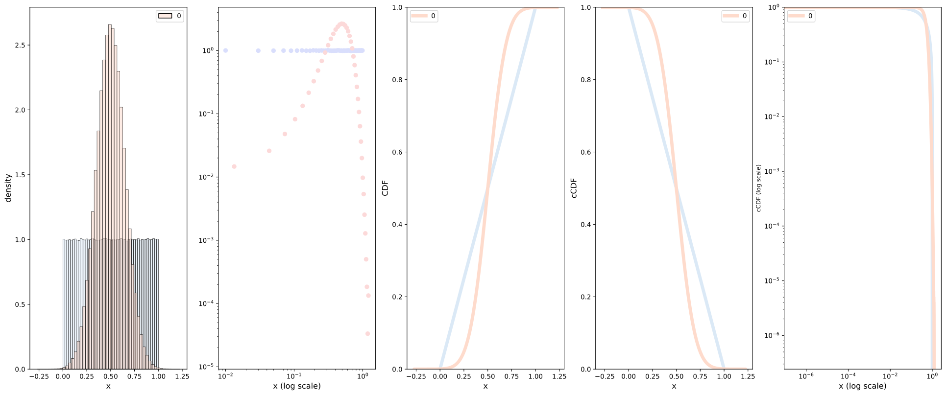
  • Again, consider a Gaussian (normal) distribution, the CFD obeys the following

  • Lets visualize on a log-log plot, for reference we also include a uniform distribution.

Power law distributions

Introduction

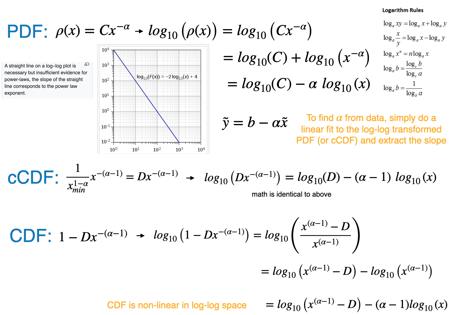
  • A power law is a functional relationship between two quantities, where a relative change in one quantity results in a relative change in the other quantity proportional to a power of the change, independent of the initial size of those quantities \[ f(x)=a x^{-k} \]
  • Example: Area of a square \(A=L \times L\), if length is doubled, the area increases by 4X

Power-law probability distributions

  • A power-law probability distribution is a distribution whose density function obeys

\[{\displaystyle P(X>x)\sim L(x)x^{-(\alpha -1)}}\]

where \(\alpha >1\) and \(L(x)\) is a slowly varying function

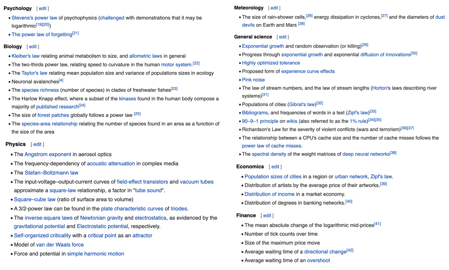
  • In real networks, properties are often power-law distributed

Source: click here

Power law examples

Source: click here

Power law:

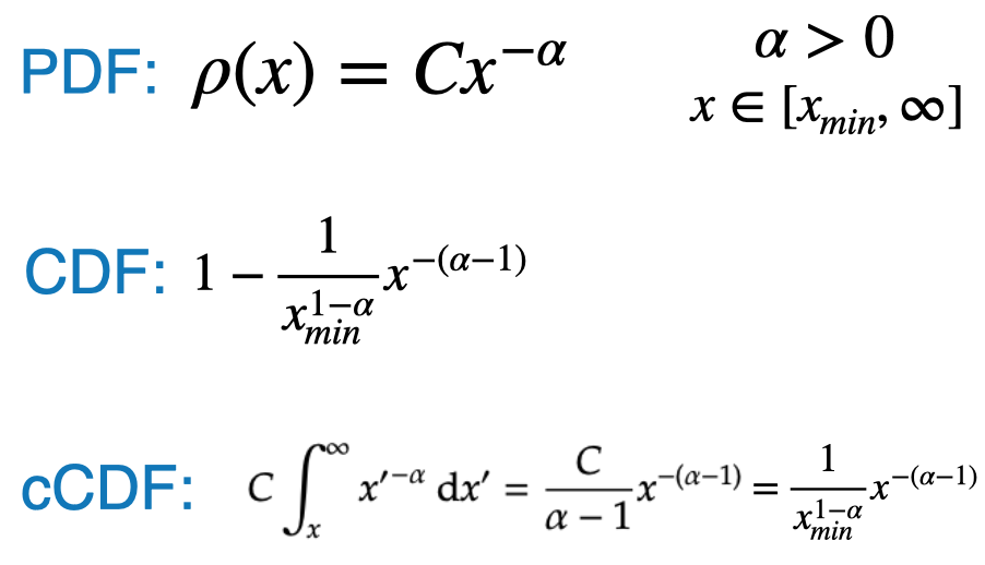
  • There are multiple ways to mathematically express a power law distribution function
  • The following is one option:
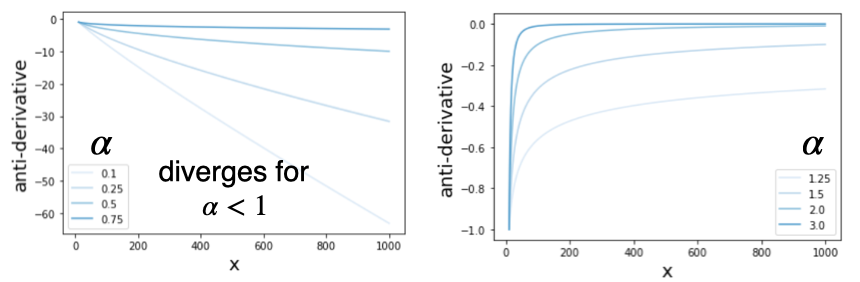
  • The anti-derivative takes the following form for different values of alpha
  • Since the function represents a probability distribution, it must have a finite integral

Exponent scaling factor

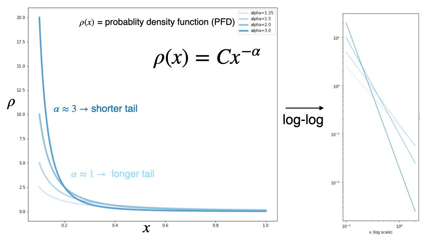
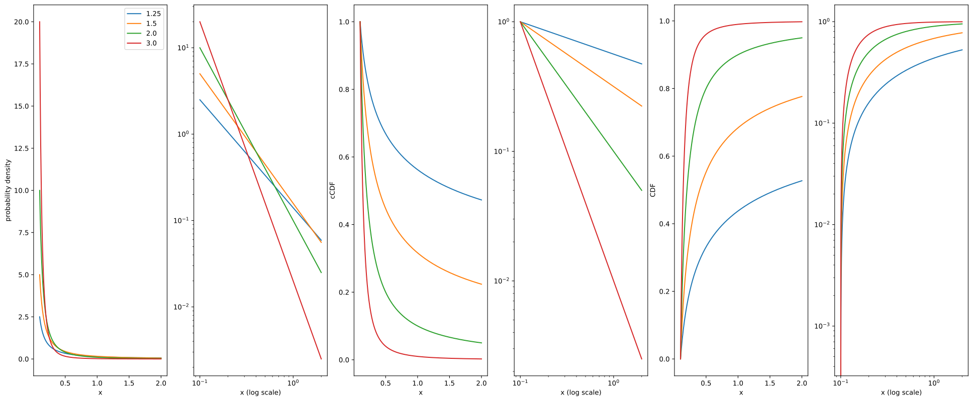
  • Here we visualize the effect of the Exponent scaling factor \(\alpha\)
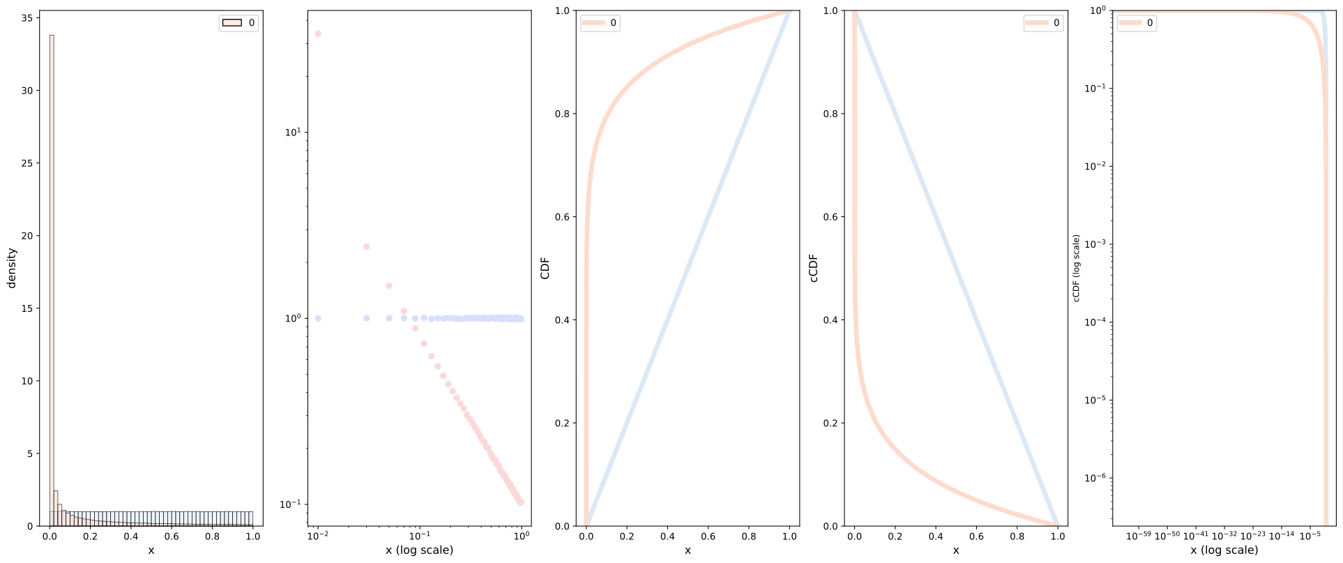
  • The straight-line on the log-log plot is often called the signature of a power law.
  • Curves which span several orders of magnitude are called broad or have a “heavy tail”

Scale invariance

  • Power laws have scale invariance, i.e the functional form doesn’t change when you scale the input
  • Given \(f(x)=a x^{-k}\), scaling the argument \(x\) by a constant factor \(c\) causes only a proportionate scaling of the function itself. \[ f(c x)=a(c x)^{-k}=c^{-k} f(x) \propto f(x) \]
  • That is, scaling by a constant \(c\) simply multiplies the original power-law relation by the constant \(c^{-k}\).
  • Thus, it follows that all power laws with a particular scaling exponent, are equivalent, up to constant factors.
  • This behavior is what produces the linear relationship when logarithms are taken of both \(f(x)\) and \(x\)
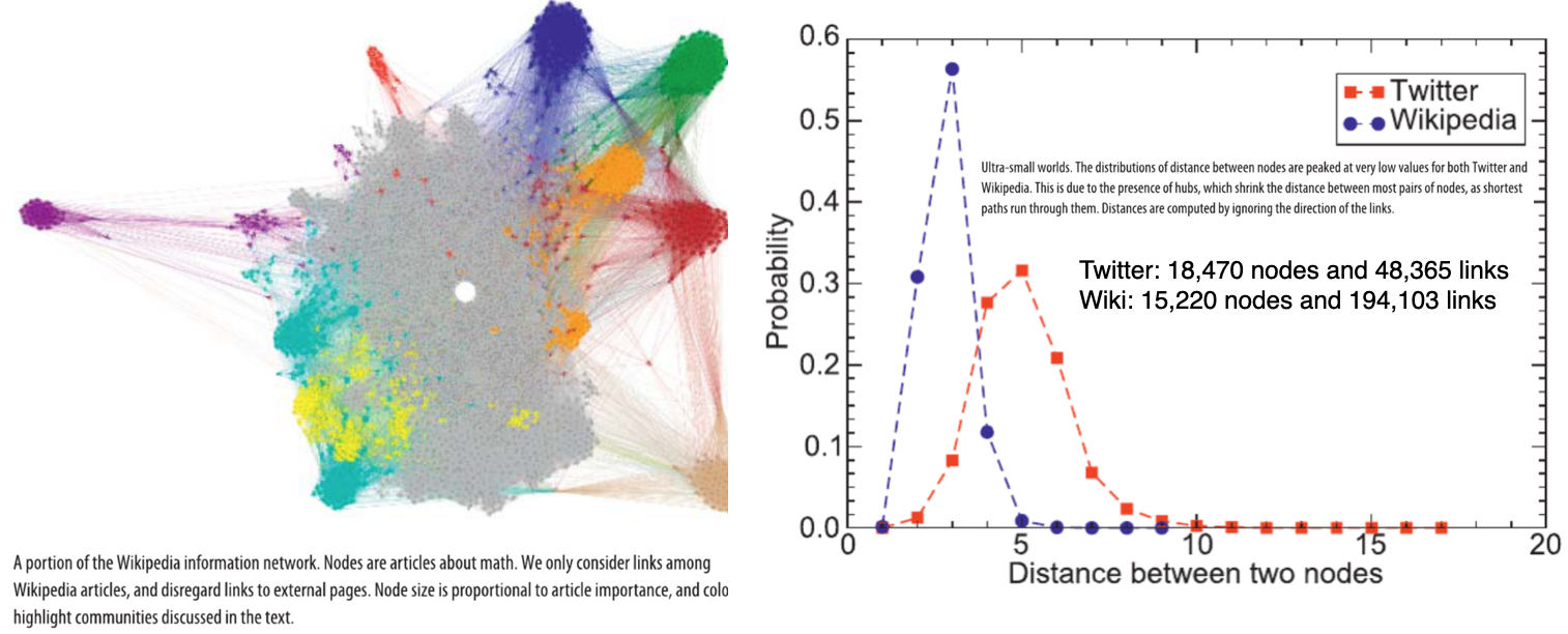
  • Networks the exhibit power-laws are sometimes called scale-free networks
Source: click here

Cumulative distribution

  • It turns out that the cumulative distribution function also follows a power law, but with a different exponent \(\alpha-1\),

Good resource: click here

Example

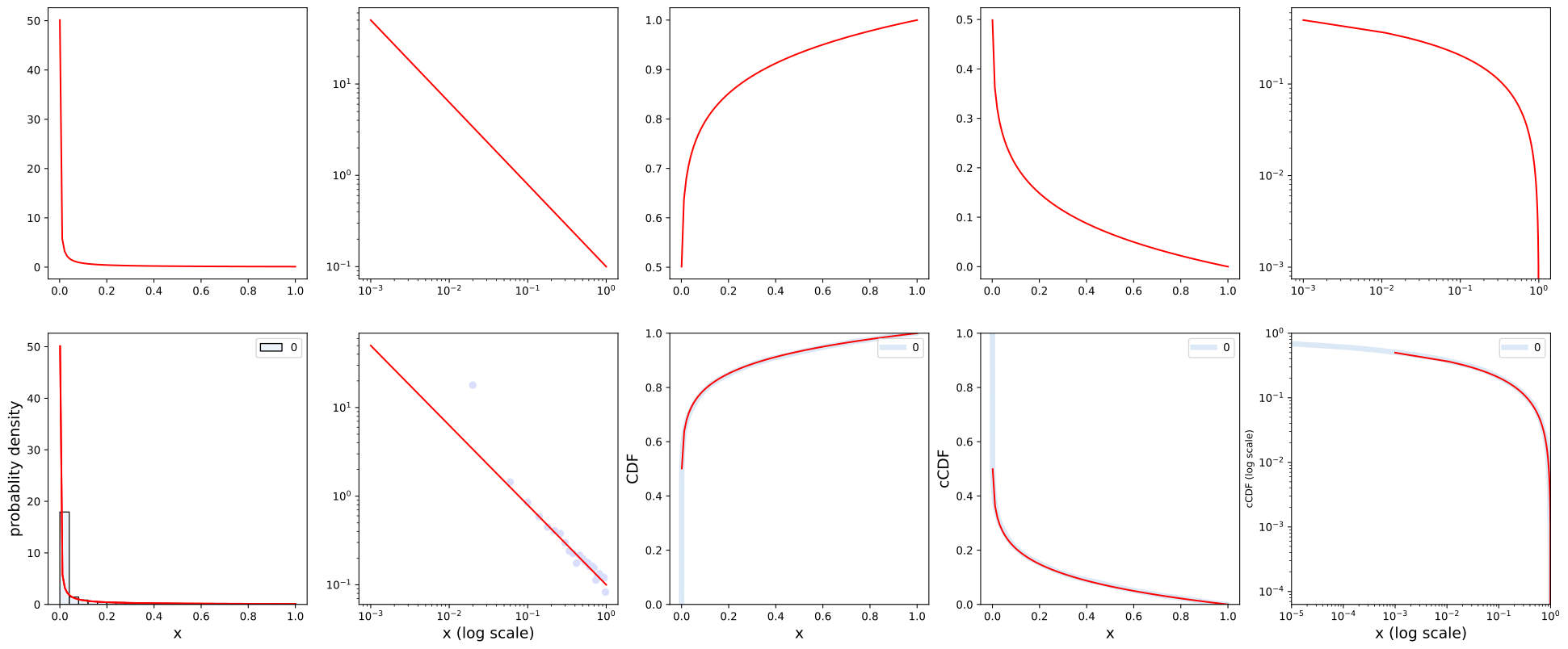
Here we show the various relevant plots for several values of \(\alpha\)

import matplotlib.pyplot as plt
import numpy as np
import seaborn as sns

#POWER LAW FORM-2
N=10000
xmin=0.1

list1=[1.25,1.5,2.0,3.0]
x1=np.linspace(xmin,2,10000)
fig, ax = plt.subplots(1,6) 
fig.set_size_inches(25, 10)
FS=10

for a in list1:
    C=(a-1)/(xmin**(1-a))
    pdf=C*x1**(-a); print(a,1-a,sum(pdf)*(x1[1]-x1[0]))
    anti_derv=C*(x1**(1-a))/(1-a)
    cdf=(C*x1**(1-a))/(a-1)

    #PDF 
    ax[0].plot(x1,pdf,"-",label=str(a))
    ax[0].legend()
    ax[0].set_xlabel("x",fontsize=FS)
    ax[0].set_ylabel("probability density",fontsize=FS)

    #PDF LOG
    ax[1].plot(x1,pdf,"-",label=str(a))
    # ax[1].legend()
    ax[1].set_xlabel("x (log scale)",fontsize=FS)
    # ax[1].set_ylabel("probability density",fontsize=FS)
    ax[1].set_xscale("log")
    ax[1].set_yscale("log")

    #ANTI
    # ax[1].plot(x1,anti_derv,"-",label=str(a))
    # ax[1].set_xlabel("x",fontsize=FS)
    # ax[1].set_ylabel("anti-derivative",fontsize=FS)

    #xCDF
    ax[2].plot(x1,cdf,"-",label=str(a))
    ax[2].set_xlabel("x",fontsize=FS)
    ax[2].set_ylabel("cCDF",fontsize=FS)

    ax[3].plot(x1,cdf,"-",label=str(a))
    ax[3].set_xlabel("x (log scale)",fontsize=FS)
    # ax[3].set_ylabel("cDF",fontsize=FS)
    ax[3].set_xscale("log")
    ax[3].set_yscale("log")


    #CDF
    ax[4].plot(x1,1-cdf,"-",label=str(a))
    ax[4].set_xlabel("x",fontsize=FS)
    ax[4].set_ylabel("CDF",fontsize=FS)

    ax[5].plot(x1,1-cdf,"-",label=str(a))
    # ax[5].plot(x1,1-x1**(-a),"-",label=str(a))
    # ax[5].plot(np.log10(x1),np.log10(1.-cdf),"-",label=str(a))
    ax[5].set_xlabel("x (log scale)",fontsize=FS)
    # ax[5].set_ylabel("cdf",fontsize=FS)
    ax[5].set_xscale("log")
    ax[5].set_yscale("log")


plt.show()
1.25 -0.25 0.5273724290711982
1.5 -0.5 0.7768737864911845
2.0 -1.0 0.9509530719583774
3.0 -2.0 0.9994022328903435

Mathematical Proofs

Alternative form

  • There are multiple ways to mathematically express a power law distribution function
  • The following is another option:

For more see: click here

Example: Code

Set up a utility function to generate the plots

import matplotlib.pyplot as plt
import numpy as np
import seaborn as sns
import warnings
warnings.filterwarnings("ignore")

N=2000000
BINS=50
FS=12

def dist_plots(x,reset=True, show_plot=True,type="density"):
    global ax,fig
    palette="Reds"; color='#fcd9d9'
    if reset:
        global fig,ax
        fig, ax = plt.subplots(1, 5) # or what ever layout you want
        fig.set_size_inches(25, 10)
        palette="Blues"; color='#d9defc'

    sns.set_palette(palette)
    
    sns.histplot(x,bins=BINS,stat=type, kde=False,ax=ax[0], color="lime")
    ax[0].set_xlabel("x",fontsize=FS)
    ax[0].set_ylabel(type,fontsize=FS)
    # ax[0].set_aspect('auto', 'box')

    #LOG PDF
    counts,bins=np.histogram(x, bins=BINS,density=False)
    bins=(np.array(bins[1:])+np.array(bins[0:-1]))/2.0
    # sns.scatterplot(x=bins,y=counts/N,palette=sns.color_palette(palette, as_cmap = True),ax=ax[1])
    if(type=="probability"): ax[1].plot(bins,counts/N,"o",c=color)
    if(type=="density"): ax[1].plot(bins,counts/N/(bins[1]-bins[0]),"o",c=color)
    ax[1].set_xscale("log")
    ax[1].set_yscale("log")
    ax[1].set_xlabel("x (log scale)",fontsize=FS)
    # ax[2].set_ylabel("Probability density",fontsize=FS)
    # ax[2].set_aspect('auto', 'box')

    #CDF
    sns.ecdfplot(data=x,ax=ax[2],linewidth=5,)
    ax[2].set_xlabel("x",fontsize=FS)
    ax[2].set_ylabel("CDF",fontsize=FS)
    # ax[2].set_xscale("log")
    # ax[2].set_yscale("log")

    #cCDF
    sns.ecdfplot(data=x,ax=ax[3],linewidth=5,complementary=True)
    ax[3].set_xlabel("x",fontsize=FS)
    ax[3].set_ylabel("cCDF",fontsize=FS)

    #LOG cCDF
    sns.ecdfplot(data=x,ax=ax[4],linewidth=5,complementary=True)
    ax[4].set_xlabel("x (log scale)",fontsize=FS)
    ax[4].set_ylabel("cCDF (log scale)",fontsize=9)
    ax[4].set_xscale("log")
    ax[4].set_yscale("log")
    # ax[4].set_xlim(0.00001,1)

    if show_plot:
        plt.show()

Case-1: Normal distribution

# print("-----------NORMAL DISTRIBUTION--------------")
x=np.random.uniform(low=0.0, high=1.0, size=(N,1))
dist_plots(x,reset=True,show_plot=False)
x=np.random.normal(0.5, 0.5*0.3, size=(N,1))
dist_plots(x,reset=False,show_plot=True)

Case-2: Power-law

# print("-----------POWER-LAW-FORM-1--------------")
x=np.random.uniform(low=0.0, high=1.0, size=(N,1))
dist_plots(x,reset=True,show_plot=False)
x=np.random.power(.1, size=(N,1))
dist_plots(x,reset=False,show_plot=True)

Case-3: Exponential distribution

# print("-----------EXPONENTIAL DISTRIBUTION--------------")
x=np.random.uniform(low=0.0, high=1.0, size=(N,1))
dist_plots(x,reset=True,show_plot=False)
x=np.random.exponential(0.05, size=(N,1))
dist_plots(x,reset=False,show_plot=True)

Power-law form-2:

import matplotlib.pyplot as plt
import numpy as np
import seaborn as sns

BINS=25
a=0.1
FS=14
N=10000
x=np.random.power(a, size=(N,1))
x1=np.linspace(.001,1,100)
pdf=a*x1**(a-1)
cdf=x1**(a)
ccdf=1.-x1**(a)

fig, ax = plt.subplots(2, 5) # or what ever layout you want
fig.set_size_inches(25, 10)
palette="Blues"; color='#d9defc'
sns.set_palette(palette)

#ANALYTIC 
ax[0,0].plot(x1,pdf,"-",c='red')

ax[0,1].plot(x1,pdf,"-",c='red')
ax[0,1].set_xscale("log")
ax[0,1].set_yscale("log")

ax[0,2].plot(x1,cdf,"-",c='red')

ax[0,3].plot(x1,ccdf,"-",c='red')

ax[0,4].plot(x1,ccdf,"-",c='red')
ax[0,4].set_xscale("log")
ax[0,4].set_yscale("log")


sns.histplot(x,bins=BINS,stat="density", kde=False,ax=ax[1,0])
ax[1,0].set_xlabel("x",fontsize=FS)
ax[1,0].plot(x1,pdf,"-",c="red")
ax[1,0].set_ylabel("probablity density",fontsize=FS)
# ax[0].set_aspect('auto', 'box')

# #LOG PDF
counts,bins=np.histogram(x, bins=BINS,density=False)
bins=(np.array(bins[1:])+np.array(bins[0:-1]))/2.0
dx=bins[1]-bins[0]
# sns.scatterplot(x=bins,y=counts/N,palette=sns.color_palette(palette, as_cmap = True),ax=ax[1,1])
ax[1,1].plot(bins,counts/N/dx,"o",c=color)
ax[1,1].set_xlabel("x (log scale)",fontsize=FS)

# #CDF
sns.ecdfplot(data=x,ax=ax[1,2],linewidth=5,)
ax[1,2].set_xlabel("x",fontsize=FS)
ax[1,2].set_ylabel("CDF",fontsize=FS)

# #cCDF
sns.ecdfplot(data=x,ax=ax[1,3],linewidth=5,complementary=True)
ax[1,3].set_xlabel("x",fontsize=FS)
ax[1,3].set_ylabel("cCDF",fontsize=FS)

# #LOG cCDF
sns.ecdfplot(data=x,ax=ax[1,4],linewidth=5,complementary=True)
ax[1,4].set_xlabel("x (log scale)",fontsize=FS)
ax[1,4].set_ylabel("cCDF (log scale)",fontsize=9)
# ax[1,4].set_xscale("log")
# ax[1,4].set_yscale("log")
ax[1,4].set_xlim(0.00001,1)

#ANALYTIC 
ax[1,0].plot(x1,pdf,"-",c='red')

ax[1,1].plot(x1,pdf,"-",c='red')
ax[1,1].set_xscale("log")
ax[1,1].set_yscale("log")

ax[1,2].plot(x1,cdf,"-",c='red')

ax[1,3].plot(x1,ccdf,"-",c='red')

ax[1,4].plot(x1,ccdf,"-",c='red')
ax[1,4].set_xscale("log")
ax[1,4].set_yscale("log")

References

Disclaimer: This document is not an original work. It contains content from many sources and is for educational purposes only.

References

1.
Menczer, F., Fortunato, S. & Davis, C. A. A first course in network science. (Cambridge University Press, 2020).