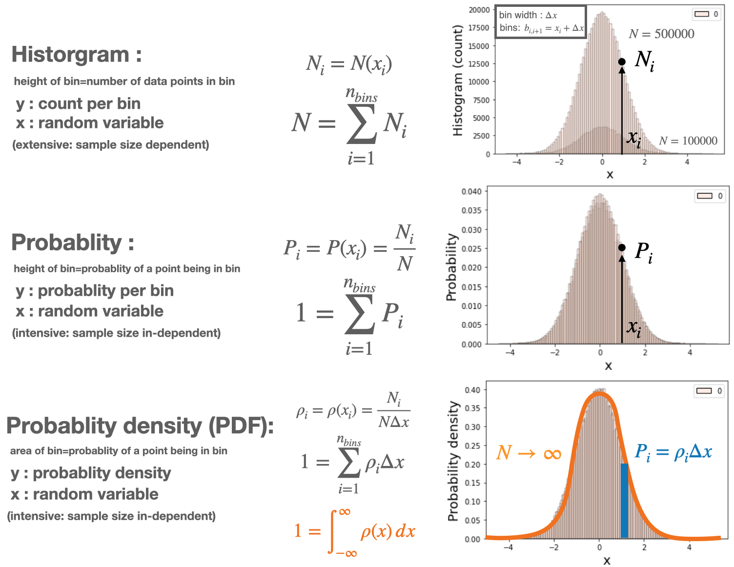
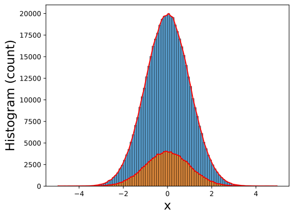
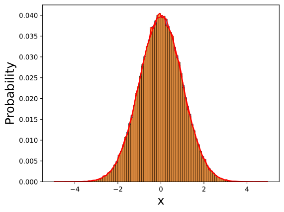
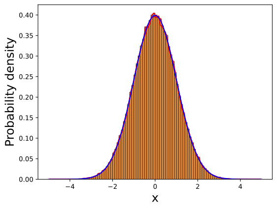
# IMPORTimport matplotlib.pyplot as pltimport numpy as npimport seaborn as sns# PARAMBINS=100FS=18u=0.0s=1.0N1=100000N2=5*N1 # GENERATE SAMPLE DATAx1=np.random.normal(u, s, size=(N1-2,1)); x1=np.append(x1,[u-5*s,u+5*s])x2=np.random.normal(u, s, size=(N2-2,1)); x2=np.append(x2,[u-5*s,u+5*s])# print(np.min(x1),np.max(x1))# print(np.min(x2),np.max(x2))# LINESPACE FOR PLOTTINGx3=np.linspace(np.min(x1),np.max(x1),100)# DIRECT CALCULATE(H1,B1)=np.histogram(x1,bins=BINS);B1=(B1[0:-1]+B1[1:])/2.0; dB1=B1[1]-B1[0] # midpoints(H2,B2)=np.histogram(x2,bins=BINS)B2=(B2[0:-1]+B2[1:])/2.0; dB2=B2[1]-B2[0] # midpoints# print(dB1, dB2)# # HISTOGRAM DISTRIBUTIONfig, ax = plt.subplots() # or what ever layout you wantsns.histplot(x2,bins=BINS,stat="count", kde=False,ax=ax)ax.plot(B2,H2,'r-')sns.histplot(x1,bins=BINS,stat="count", kde=False,ax=ax)ax.plot(B1,H1,'r-')ax.set_xlabel("x",fontsize=FS)ax.set_ylabel("Histogram (count)",fontsize=FS)plt.show()# # # PROBABILITY (LIKELIHOOD) DISTRIBUTIONfig, ax = plt.subplots() # or what ever layout you wantsns.histplot(x2,bins=BINS,stat="probability", kde=False,ax=ax)ax.plot(B2,H2/N2,'r-')sns.histplot(x1,bins=BINS,stat="probability", kde=False,ax=ax)ax.plot(B1,H1/N1,'r-')ax.set_xlabel("x",fontsize=FS)ax.set_ylabel("Probability",fontsize=FS)plt.show()# # # PROBABILITY DENSITY DISTRIBUTIONfig, ax = plt.subplots() # or what ever layout you wantsns.histplot(x1,bins=BINS,stat="density", kde=False,ax=ax)ax.plot(B2,H2/N2/dB2,'r-')sns.histplot(x2,bins=BINS,stat="density", kde=False,ax=ax)ax.plot(B1,H1/N1/dB1,'r-')ax.set_xlabel("x",fontsize=FS)ax.plot(x3,np.exp(-0.5*((x3-u)/s)**2.0)/(2.*np.pi*s)**0.5,'b-')ax.set_ylabel("Probability density",fontsize=FS)plt.show()
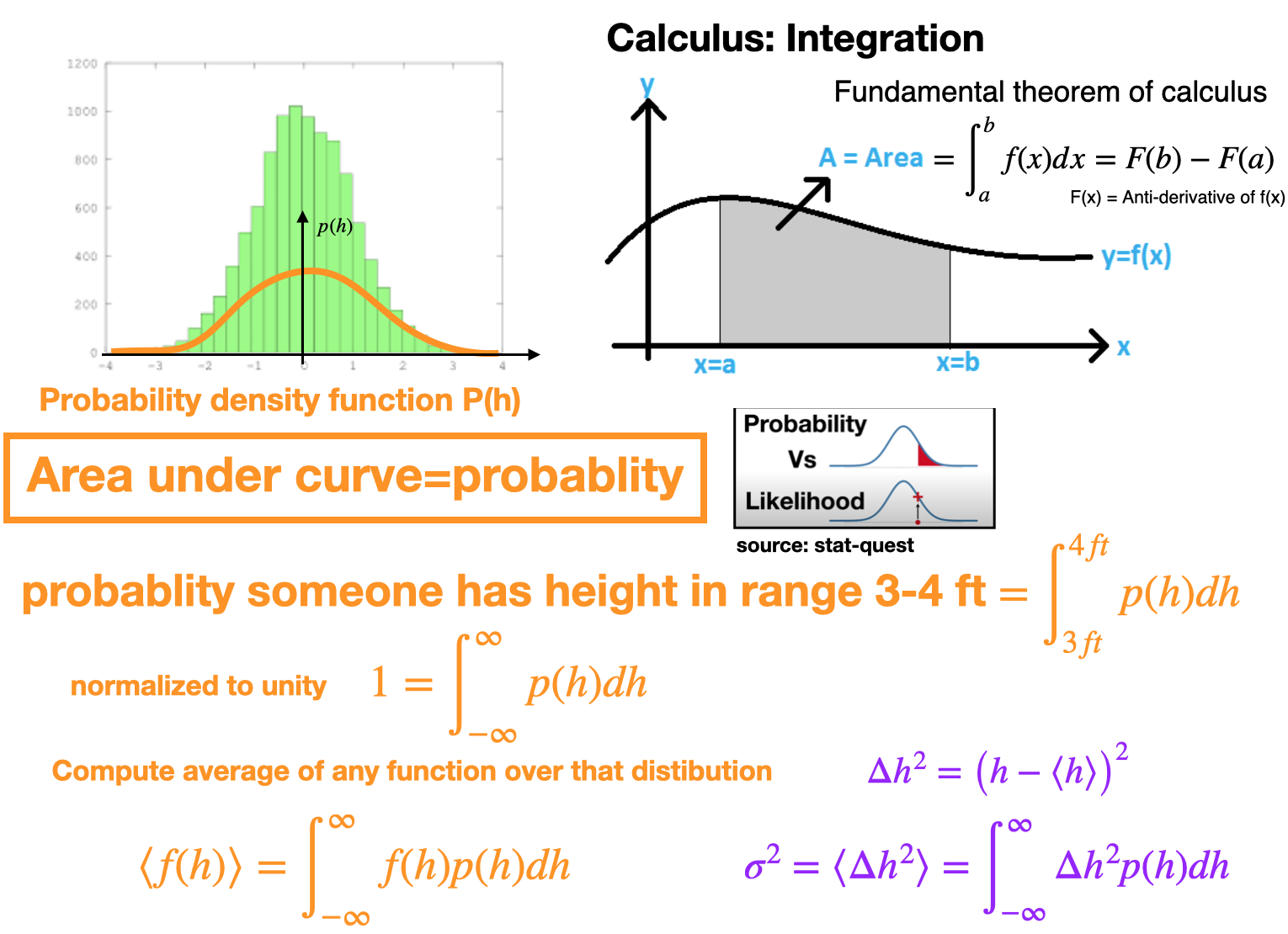
Probability density function
Cumulative distributions (CDF)
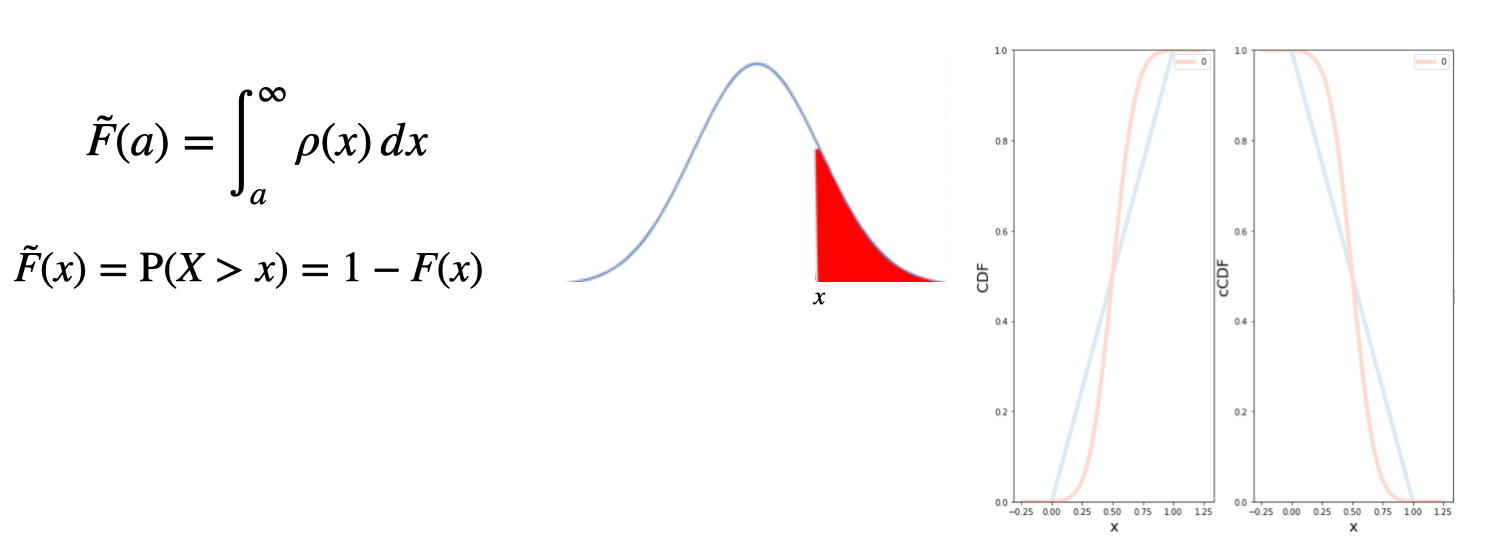
The Cumulative distribution function (CDF) of a continuous random variable \(X\) can be expressed as the integral of its probability density function \(f_X\) as \(F(a)=\int _{-\infty }^{a}\rho(x)\,dx\)
Complementary CDF: (cCDF)
Complementary cumulative distribution function (tail distribution)
Sometimes, it is useful to study the opposite question and ask how often the random variable is above a particular level.
This is called the complementary cumulative distribution function (ccdf) or simply the tail distribution or exceedance, and is defined as
Log-log plots
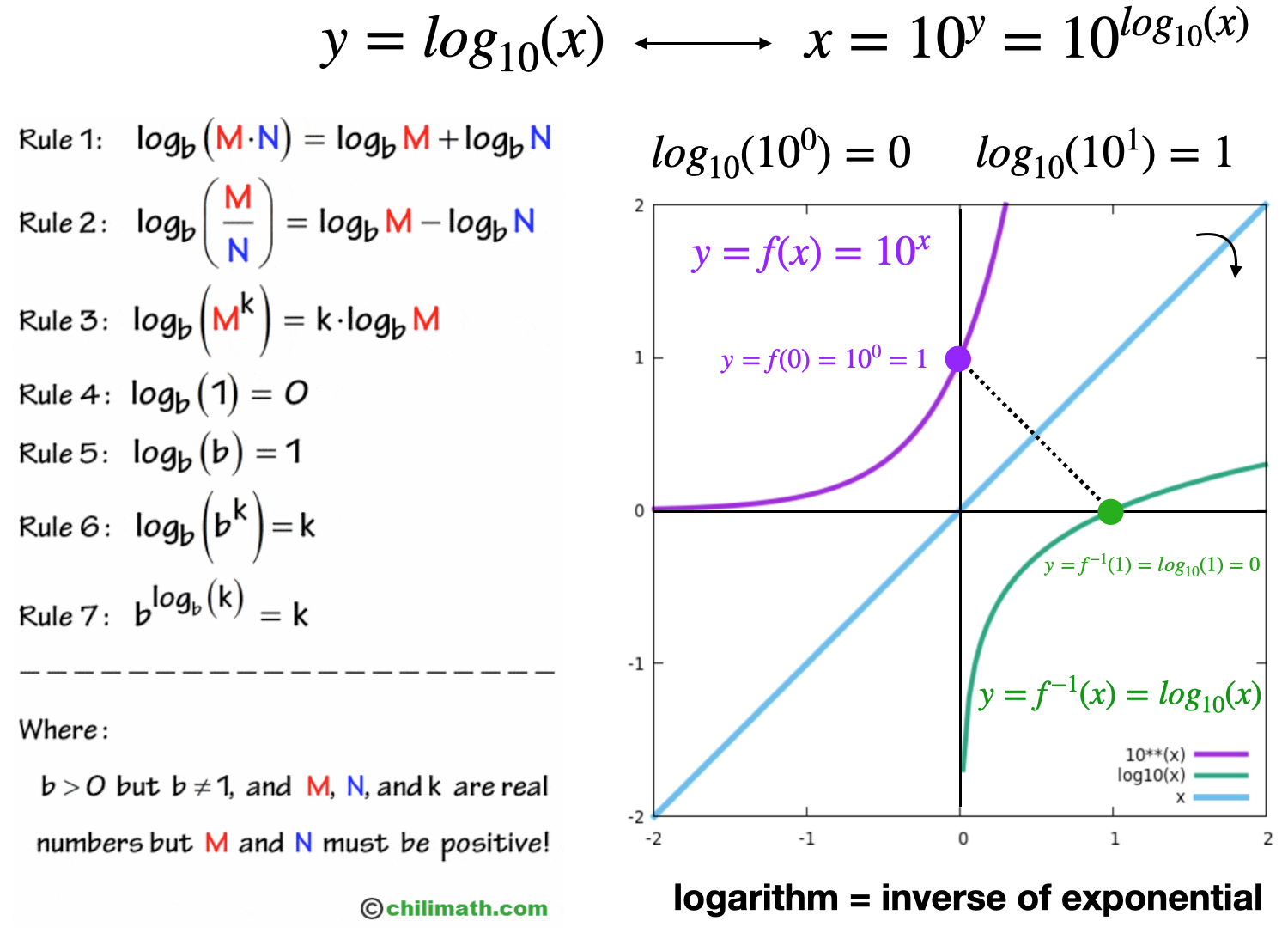
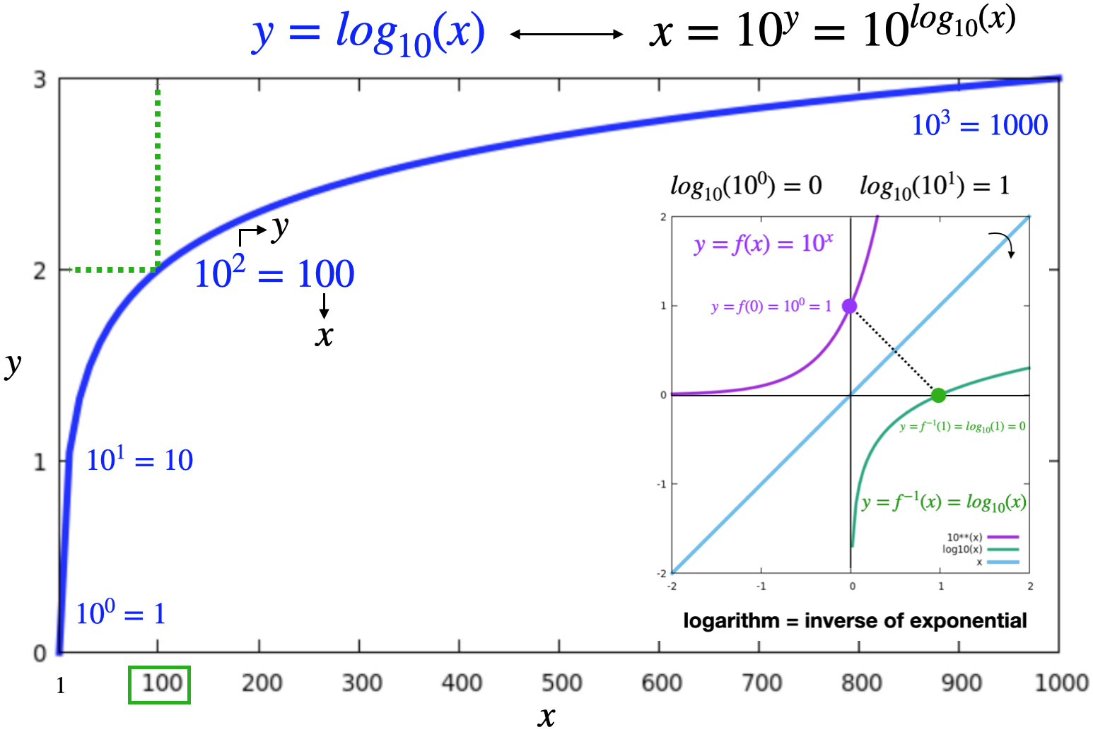
Recall: Logarithms
Recall: Logarithms
Log-scale
In network analysis, often we plot network quantities distributions on a log-log scale
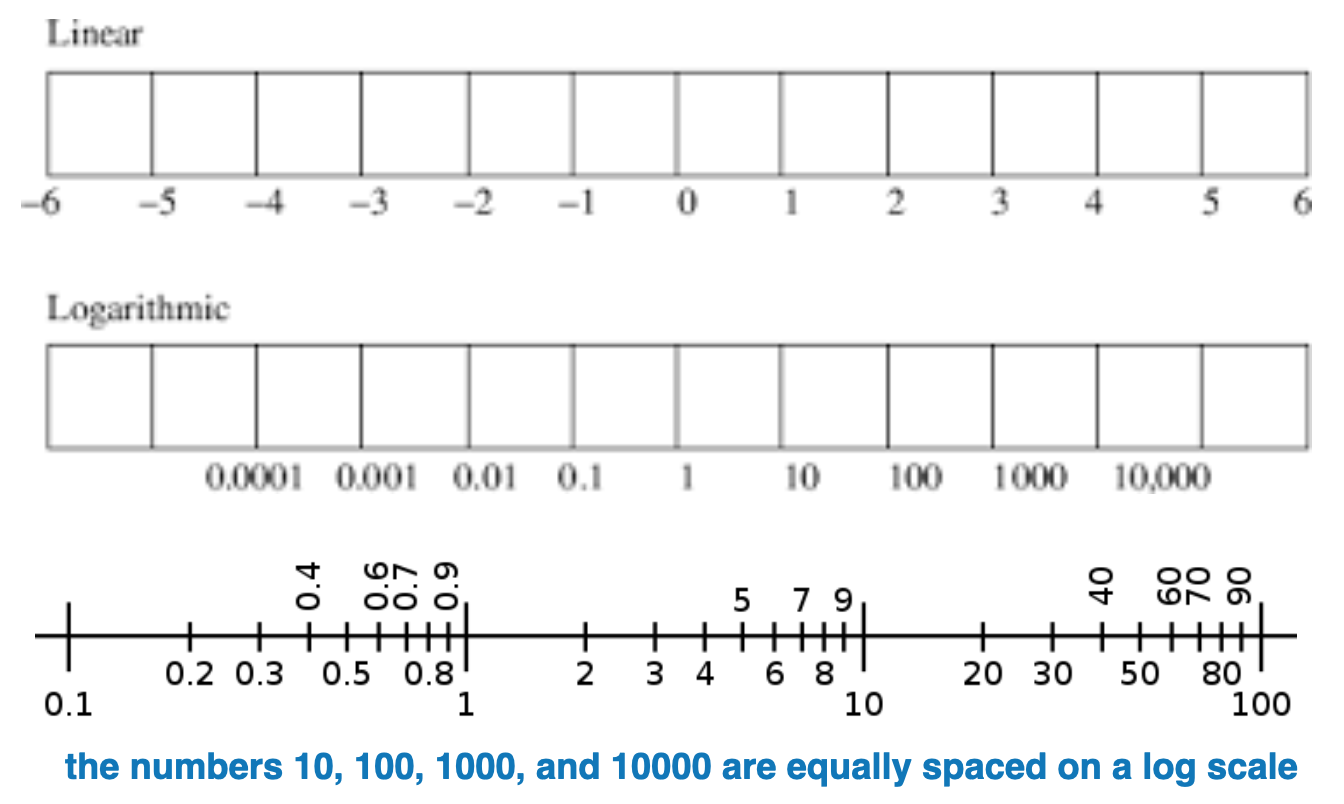
A logarithmic scale (or log scale) is a way of displaying numerical data over a very wide range of values in a compact way—typically the largest numbers in the data are hundreds or even thousands of times larger than the smallest numbers
Linear scale: Equal changes in data result in EQUAL differences in length encoding
Log-scale: Equal changes in data result in NON-EQUAL differences in length
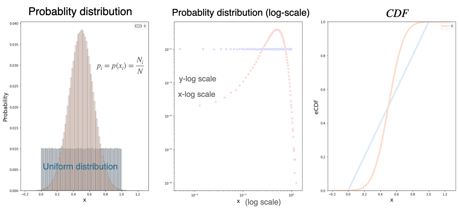
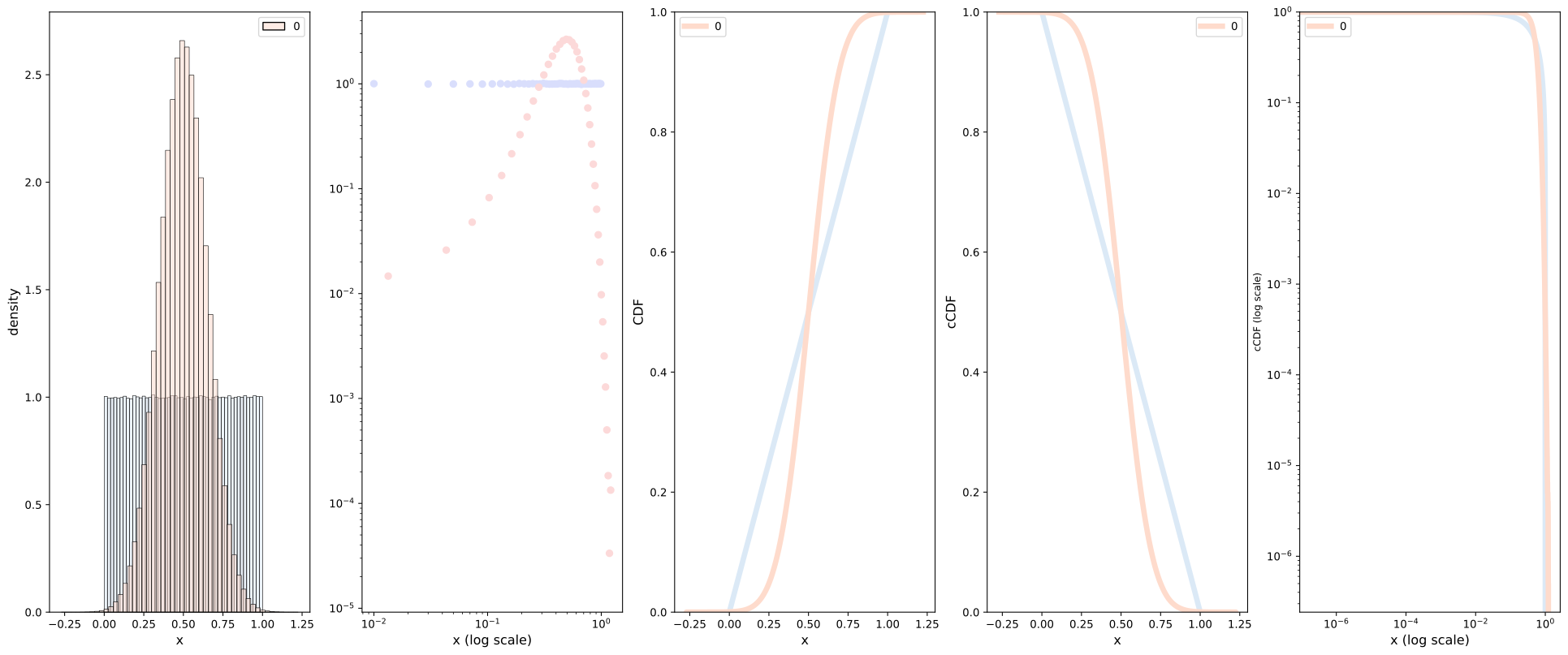
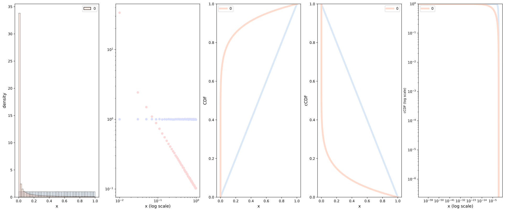
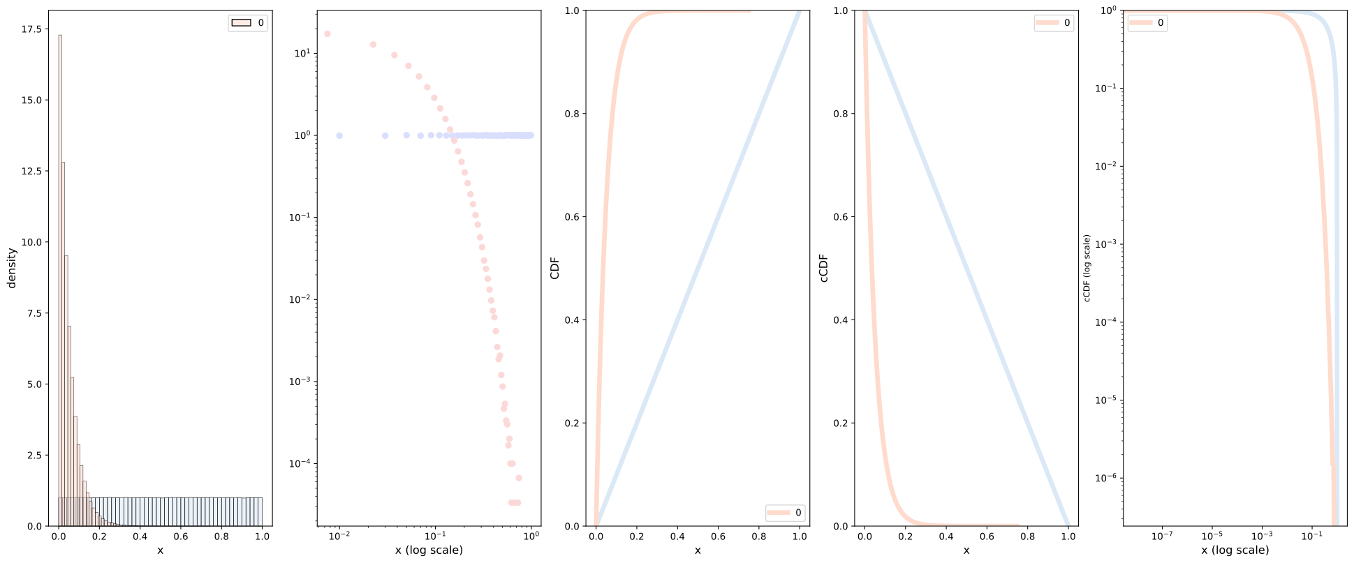
Again, consider a Gaussian (normal) distribution, the CFD obeys the following
Lets visualize on a log-log plot, for reference we also include a uniform distribution.
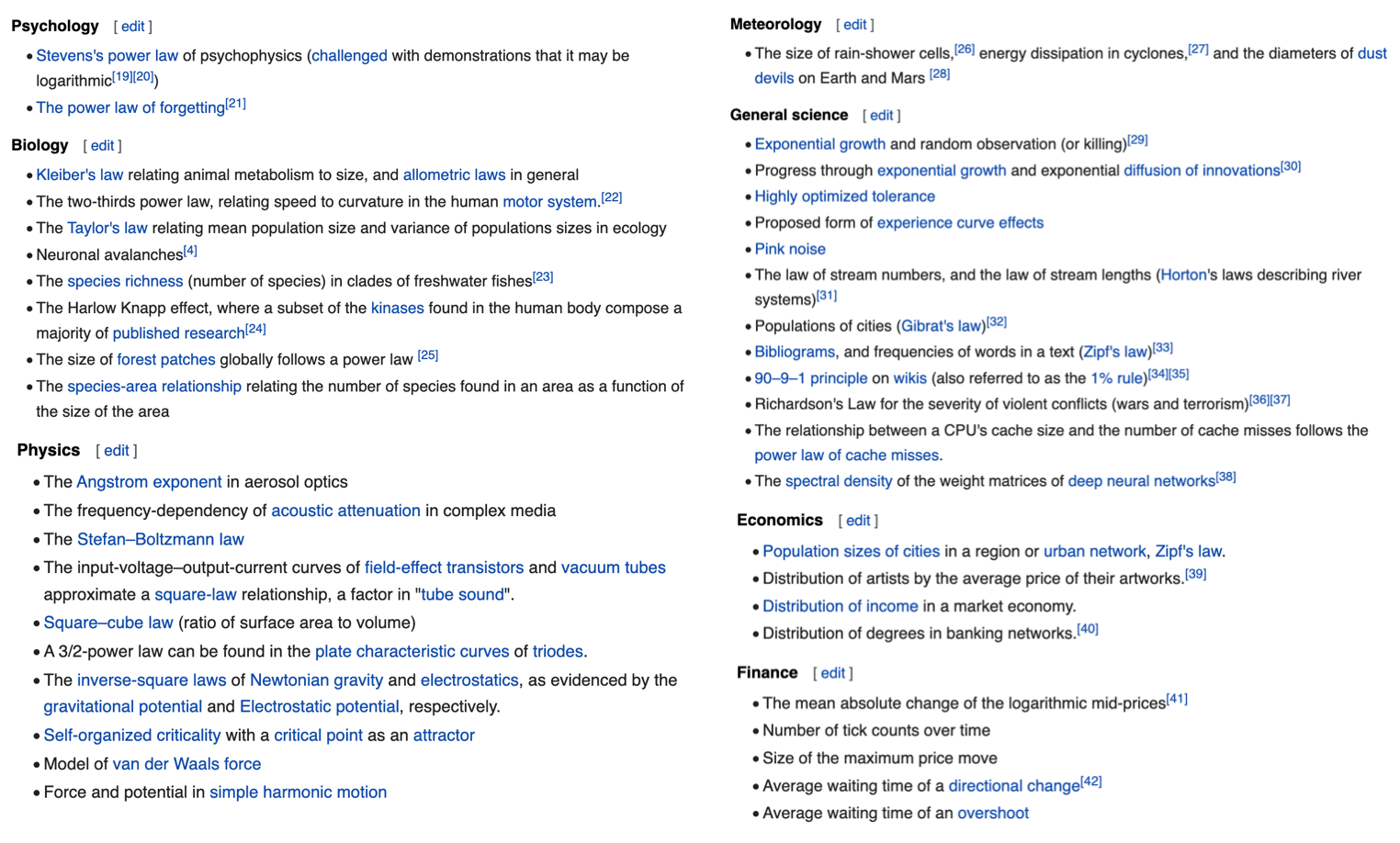
Power law distributions
Introduction
A power law is a functional relationship between two quantities, where a relative change in one quantity results in a relative change in the other quantity proportional to a power of the change, independent of the initial size of those quantities \[ f(x)=a x^{-k} \]
Example: Area of a square \(A=L \times L\), if length is doubled, the area increases by 4X
Power-law probability distributions
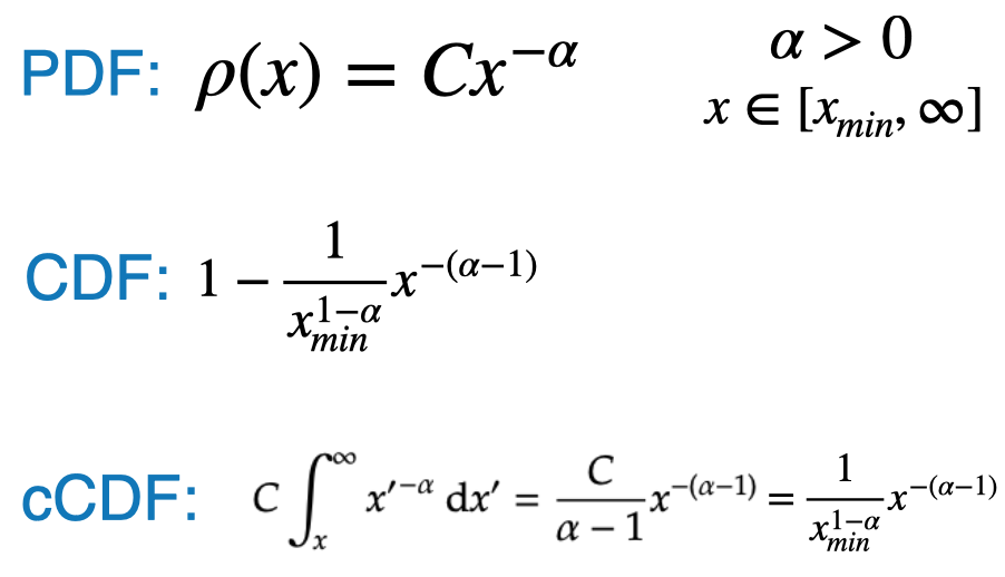
A power-law probability distribution is a distribution whose density function obeys
There are multiple ways to mathematically express a power law distribution function
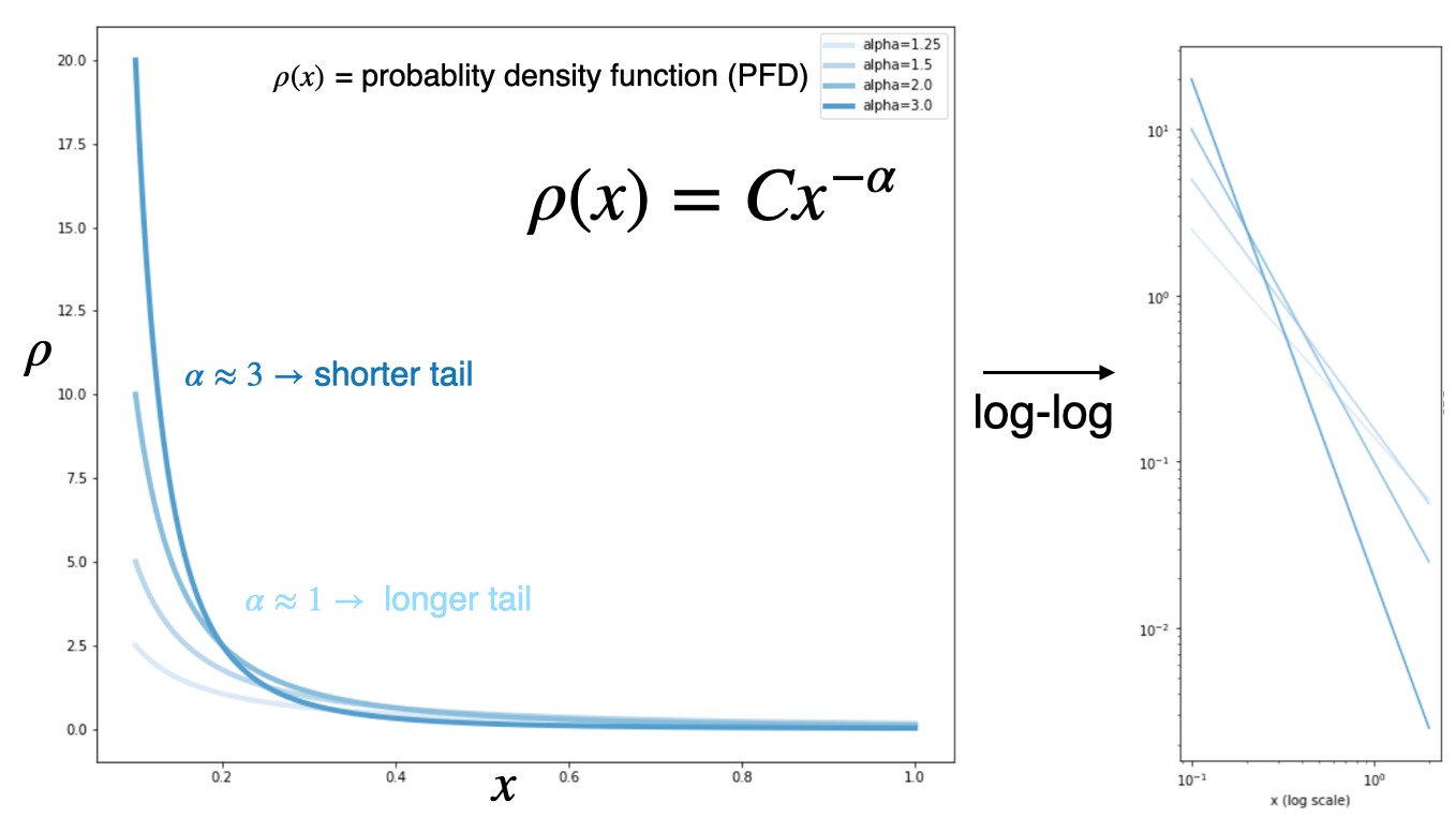
The following is one option:
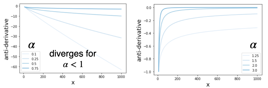
The anti-derivative takes the following form for different values of alpha
Since the function represents a probability distribution, it must have a finite integral
Exponent scaling factor
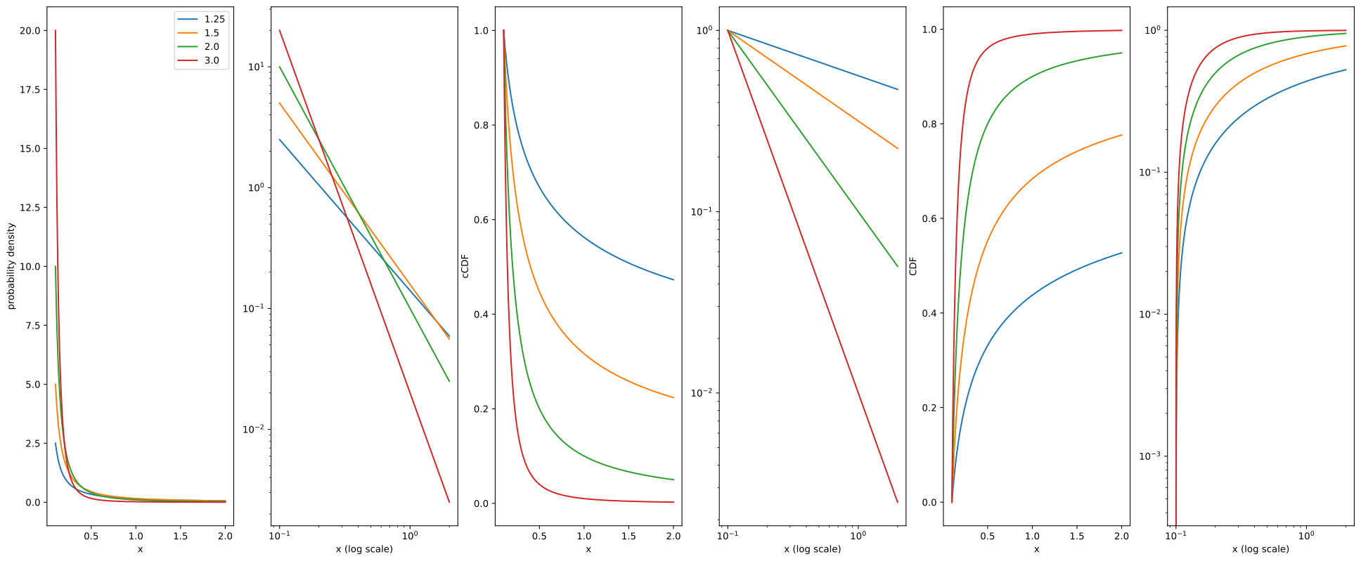
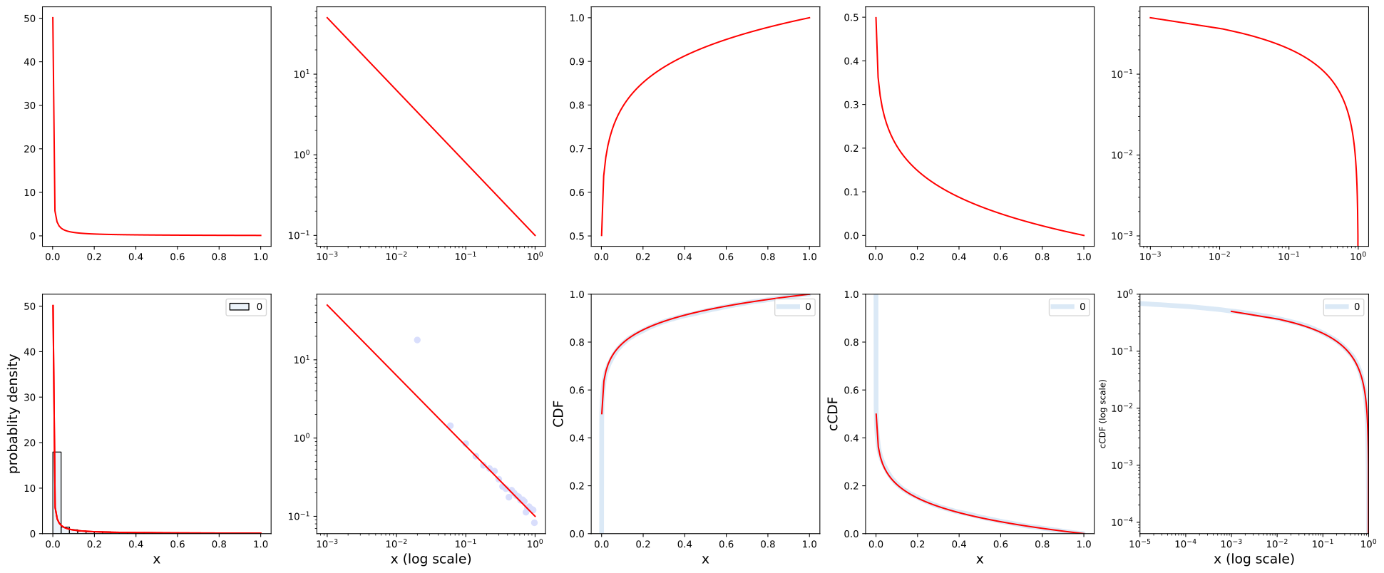
Here we visualize the effect of the Exponent scaling factor \(\alpha\)
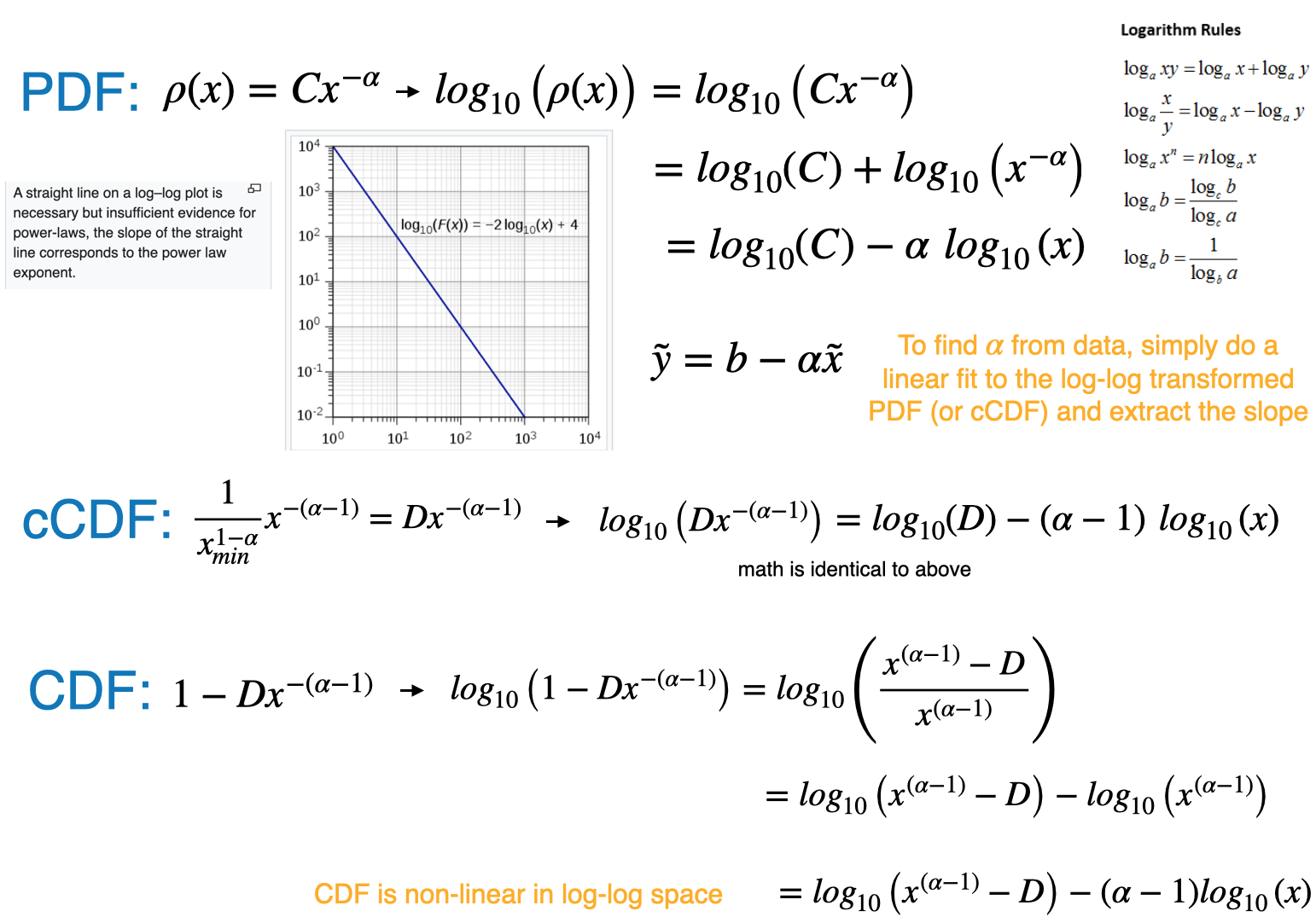
The straight-line on the log-log plot is often called the signature of a power law.
Curves which span several orders of magnitude are called broad or have a “heavy tail”
Scale invariance
Power laws have scale invariance, i.e the functional form doesn’t change when you scale the input
Given \(f(x)=a x^{-k}\), scaling the argument \(x\) by a constant factor \(c\) causes only a proportionate scaling of the function itself. \[
f(c x)=a(c x)^{-k}=c^{-k} f(x) \propto f(x)
\]
That is, scaling by a constant \(c\) simply multiplies the original power-law relation by the constant \(c^{-k}\).
Thus, it follows that all power laws with a particular scaling exponent, are equivalent, up to constant factors.
This behavior is what produces the linear relationship when logarithms are taken of both \(f(x)\) and \(x\)
Networks the exhibit power-laws are sometimes called scale-free networks