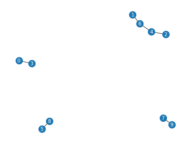
Core Decomposition Definition: A method to decompose a network into nested subgraphs, called k-cores, where each node is connected to at least k other nodes within the subgraph.
K-Core: A maximal subgraph in which each vertex has at least degree k.
Importance: Helps identify central and cohesive areas in a network.
Algorithm: Typically involves iteratively removing nodes with degrees less than k until no such nodes remain.
Applications: Used in social network analysis, biology, computer networks, and more to reveal the structure and hierarchies within networks.
Use-case: Visualizing the core
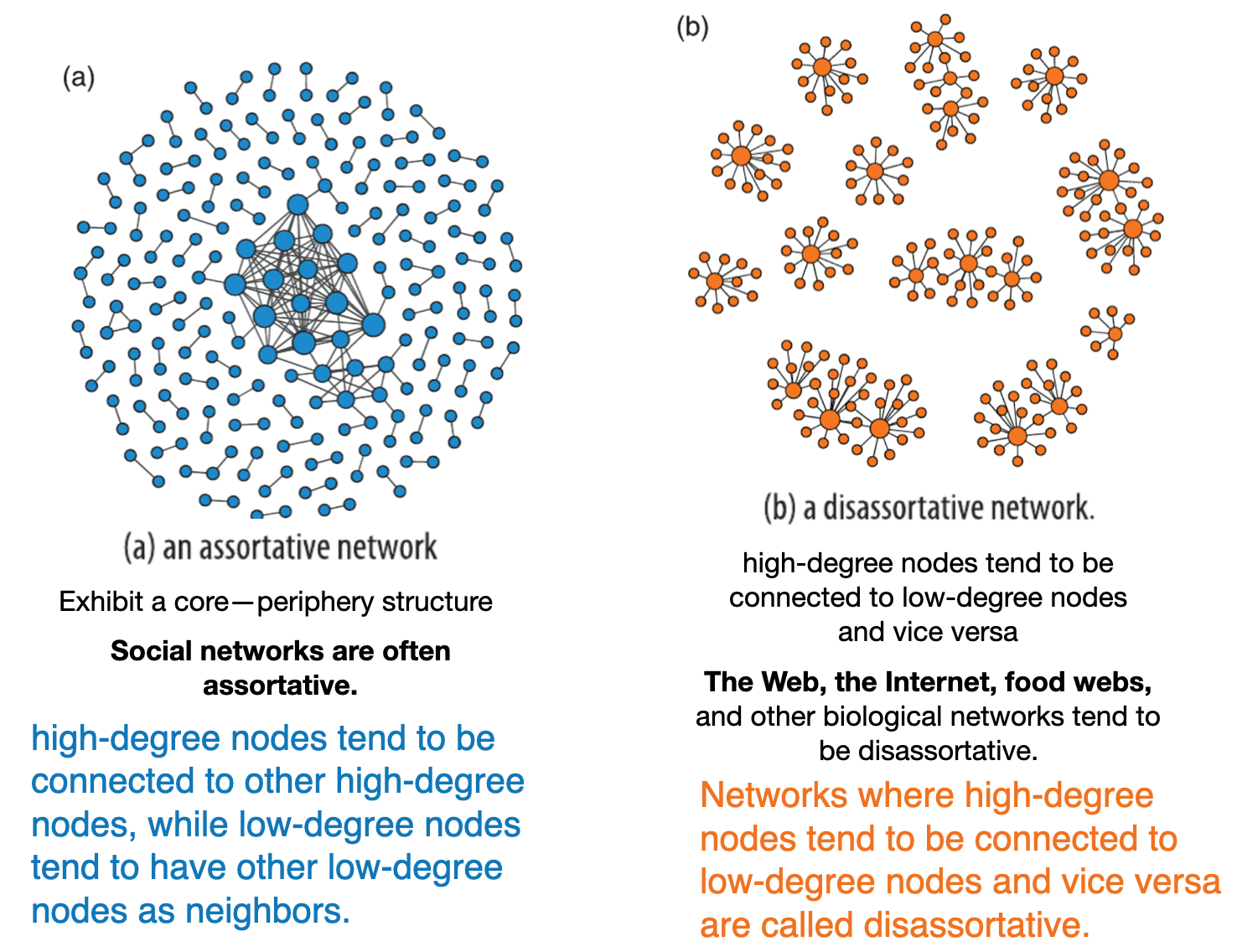
When analyzing or visualizing a large network, it is often useful to focus on its denser portion (the core)
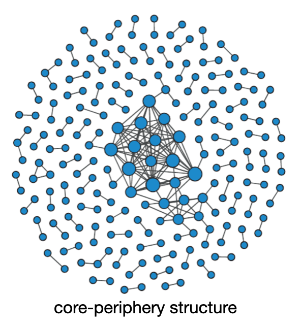
Degree shells: The degree can be used to separate a network into distinct portions, called shells, based on their position in the core
Low-degree: outer shells on the periphery.
High-degree: core nodes
As low degree nodes are removed, what remains is a denser and denser sub-network (i.e. the core)
Core decomposition is particularly helpful in practice for filtering out peripheral nodes when visualizing large networks.
Core decomposition algorithm
Formally, the \(k\)-core decomposition algorithm starts by setting \(k=0\). Then it proceeds iteratively. Each iteration corresponds to a value of \(k\) and consists of a few simple steps:
Recursively remove all nodes of degree \(k\), until there are no more left.
The removed nodes make up the \(k\)-shell and the remaining nodes make up the \((k+\) 1)-core, because they all have degree \(k+1\) or larger.
If there are no nodes left in the core, terminate; else, increment \(k\) for the next iteration.
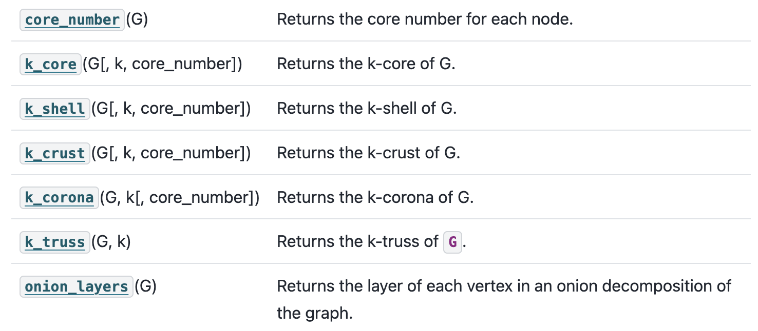
NetworkX has functions for core decomposition:
Example: Political network
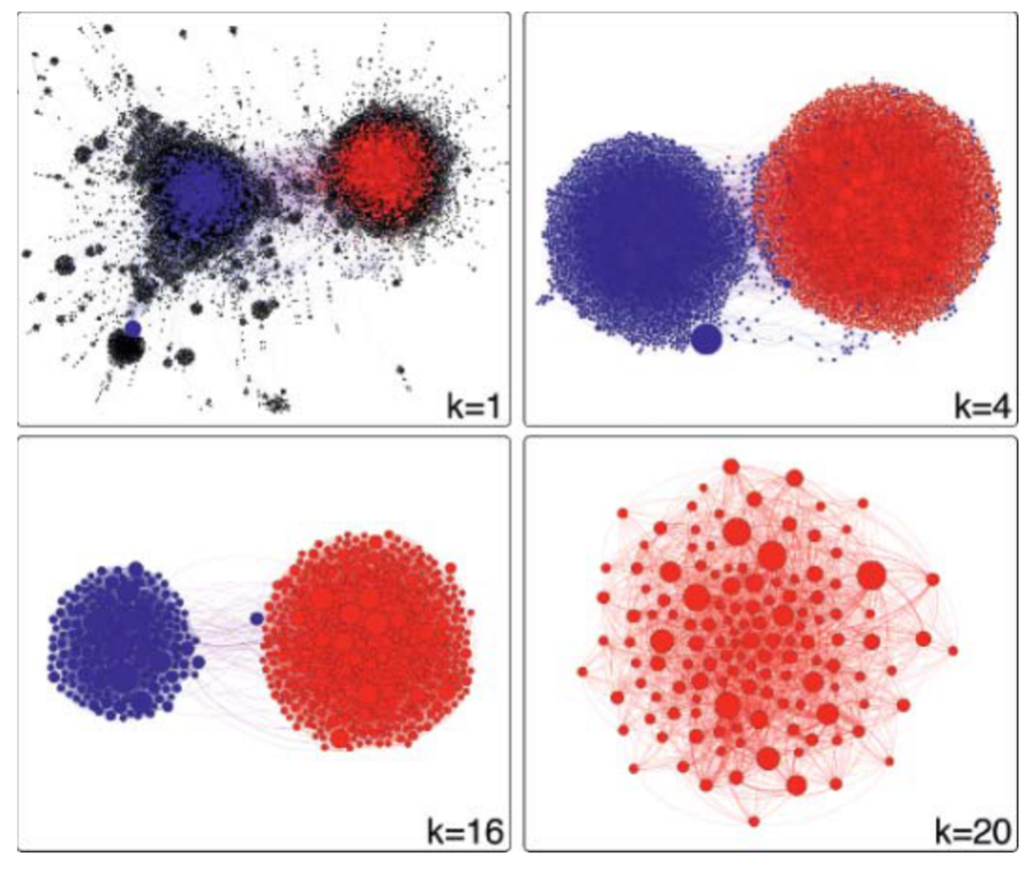
Filtering by \(k\)-core decomposition. We start from the full Twitter political retweet network \((k=1)\).
As we increase \(k\), peripheral nodes are removed and the remaining core becomes smaller and denser.
The innermost core contains only red nodes, corresponding to conservative accounts; each has at least \(k=20\) neighbors.
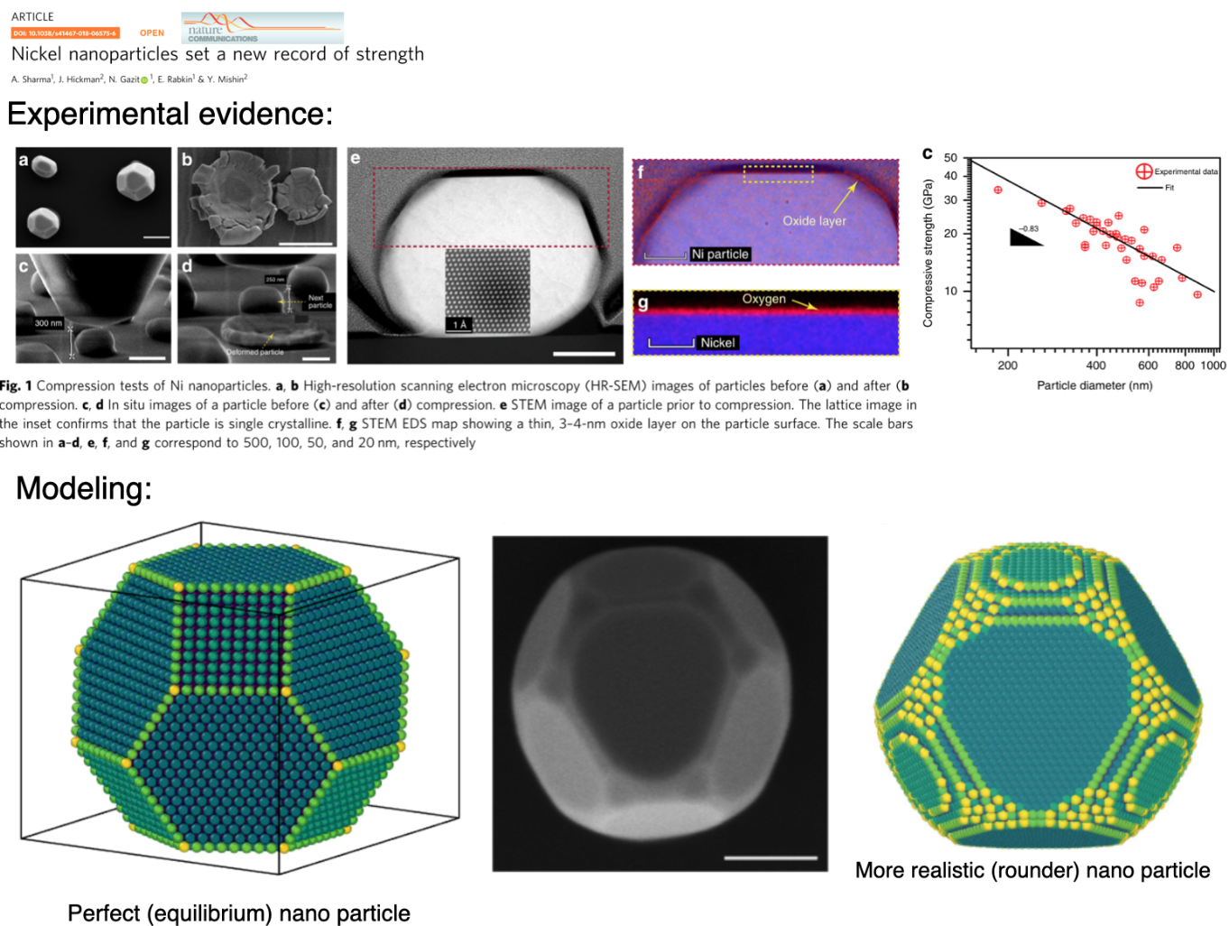
Example: Physical network
Code example
Recall relevant functions
Utility function
Code
import networkx as nximport matplotlib.pyplot as plt#FUNCTION FOR NETWORK PLOTTING # def draw_network(G):# #CUSTOMIZE GRAPH A BIT# pos= nx.circular_layout(G)# nx.draw(G,# with_labels=True,# node_color='blue',# node_size=1600,# pos=pos,# font_color='white',# font_size=16,# )# plt.show()def draw_network(G):#COMPUTE DEGREE: --> "LIST" WITH NODE DEGREES G_DEGREE=G.degree();#print(G_DEGREE,G_DEGREE[5],type(G_DEGREE)) # #LABELS (DICT)# labels={}# for n,d in G_DEGREE: labels[n]=d #str(n)+"-"+str(d) #SORT DEGREE AND STORE IN LIST degree_sequence =sorted((d for n, d in G_DEGREE), reverse=True) dmax =max(degree_sequence) #MAX DEGREE#INITIALIZE MPL FIGURE+AX fig = plt.figure("Degree of a random graph", figsize=(12, 12))# Create a gridspec for adding subplots of different sizes axgrid = fig.add_gridspec(5, 4)#PLOT NETWORK IN UPPER GRID SPACES ax0 = fig.add_subplot(axgrid[0:3, :])# pos = nx.spring_layout(G)# pos= nx.circular_layout(G) nx.draw(G, with_labels=True,# labels=labels, node_color='blue', node_size=500, font_color='white', font_size=16, pos=pos,ax=ax0 ) ax0.set_title("Network Graph: G")#PLOT RANK (IMPORTANCE BASED ON DEGREE) VS DEGREE) ax1 = fig.add_subplot(axgrid[3:, :2]) ax1.plot(degree_sequence, "b-", marker="o") ax1.set_title("Degree Rank Plot") ax1.set_ylabel("Degree") ax1.set_xlabel("Rank")#PLOT RANK HISTOGRAM ax2 = fig.add_subplot(axgrid[3:, 2:]) ax2.bar(*np.unique(degree_sequence, return_counts=True)) ax2.set_title("Degree histogram") ax2.set_xlabel("Degree") ax2.set_ylabel("# of Nodes") ax0.set_aspect('equal', 'box') fig.tight_layout() plt.show()
Create and visualize network
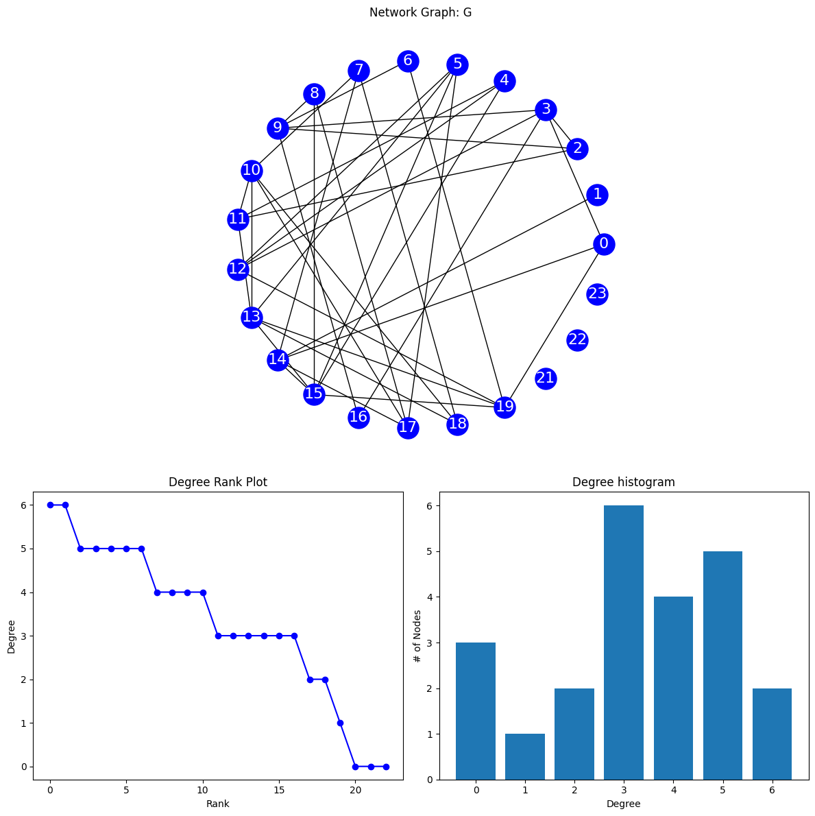
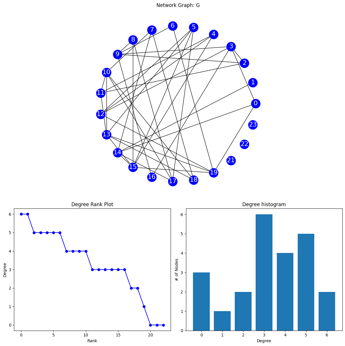
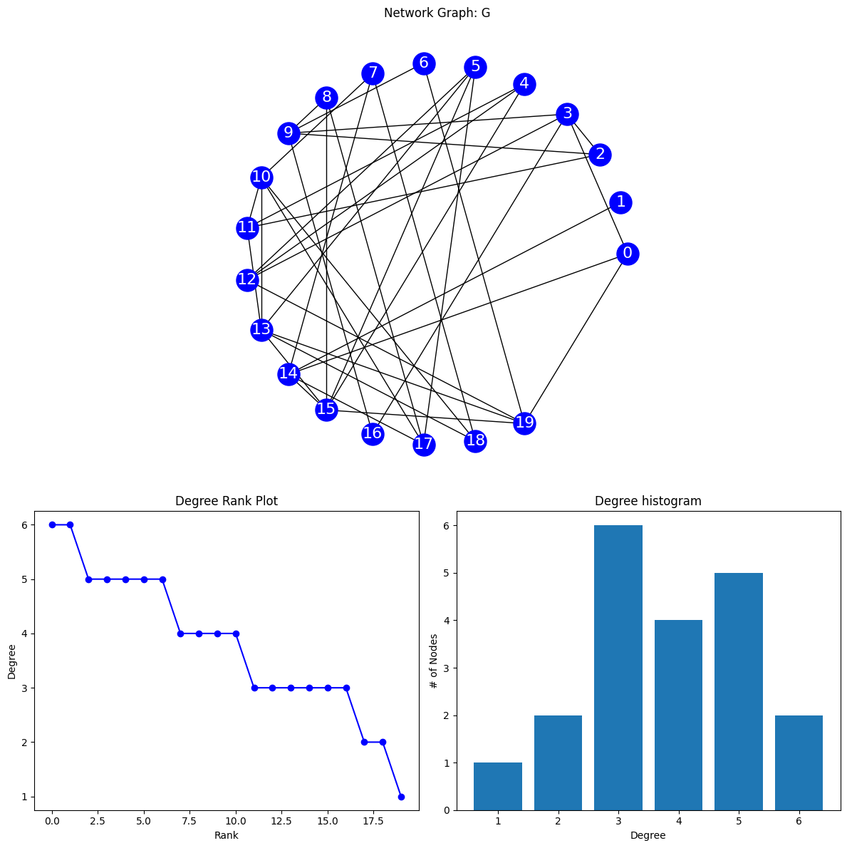
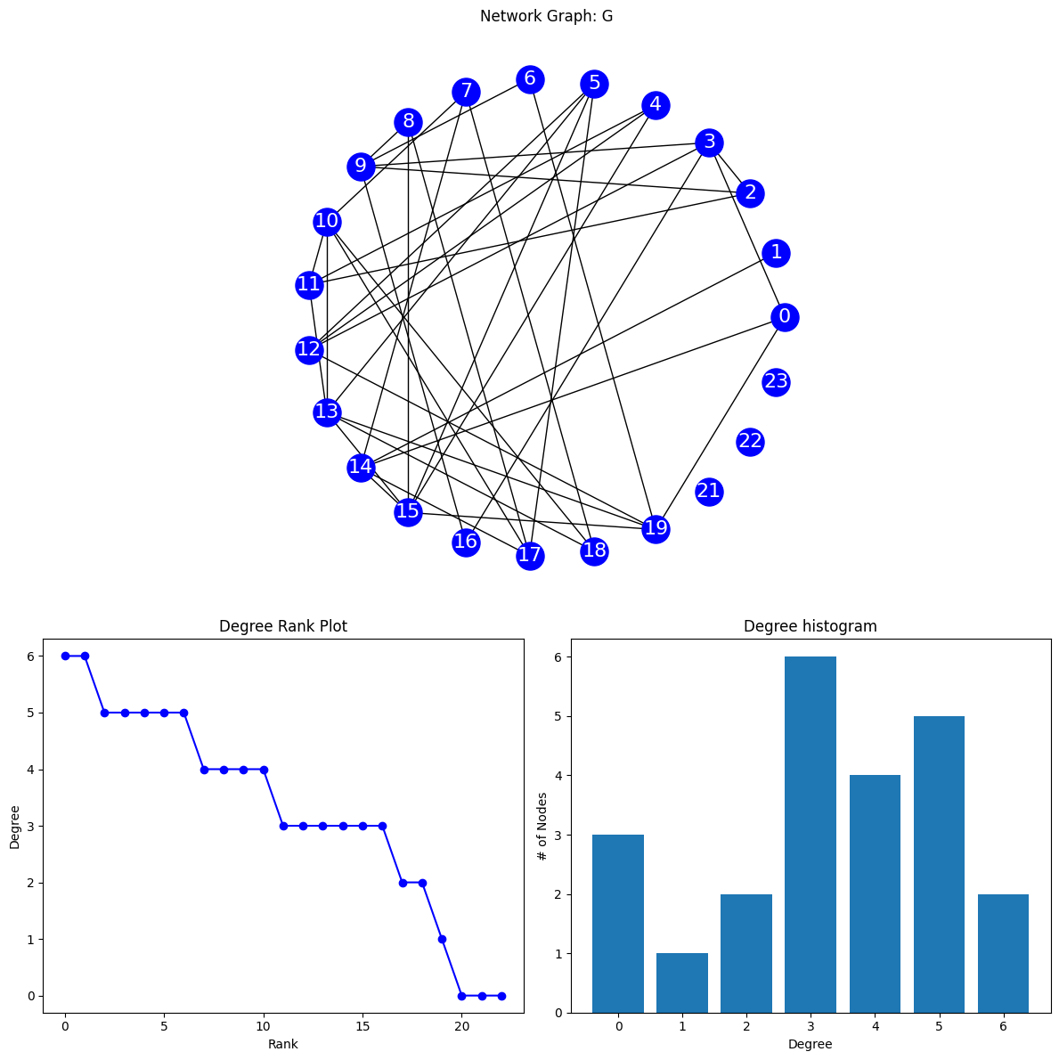
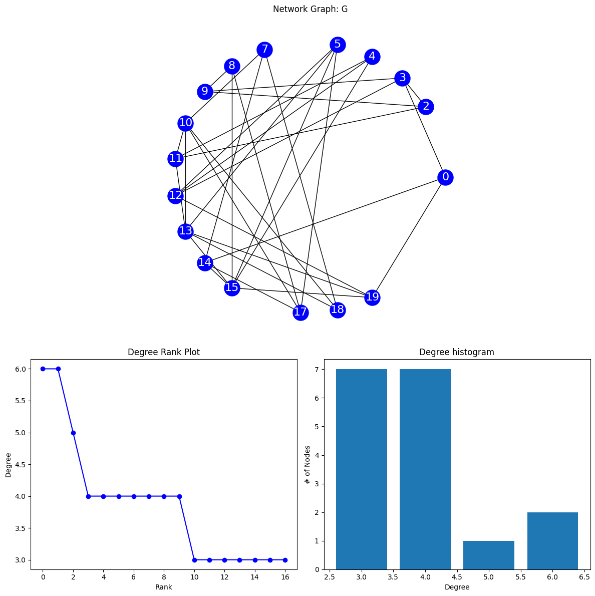
Lets start with a random network with a density of 0.2 and add some singletons
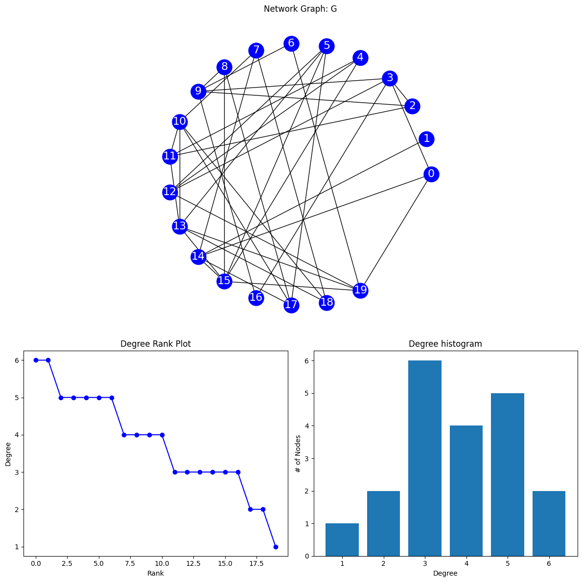
Notice how this is the same as K=1 (since removing the singletons leaves the GCC in this case)
Code
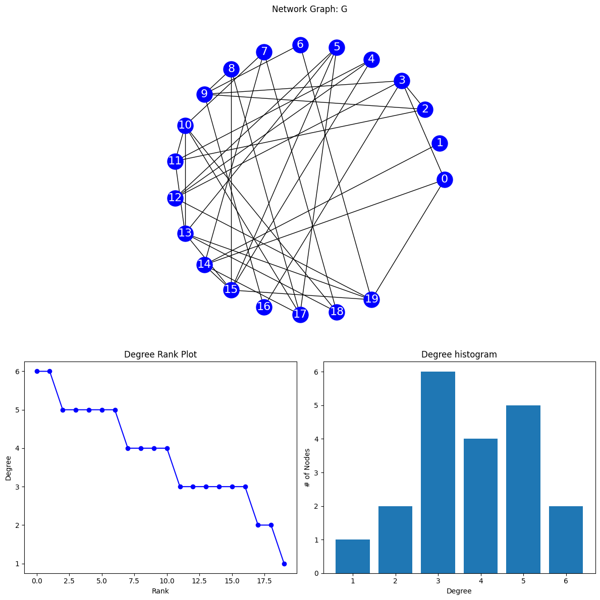
def isolate_GCC(G):# get list of CC and return the first one in sorted list, i.e the larges one comps =sorted(nx.connected_components(G),key=len, reverse=True) nodes_in_giant_comp = comps[0]# return subgraphreturn nx.subgraph(G, nodes_in_giant_comp)GCC=isolate_GCC(G)draw_network(GCC)
Core example: K=2
Code
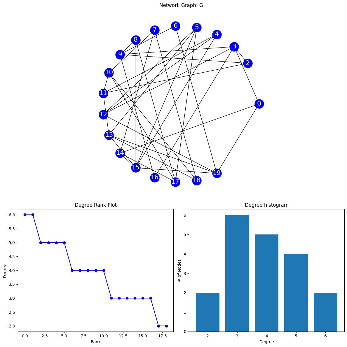
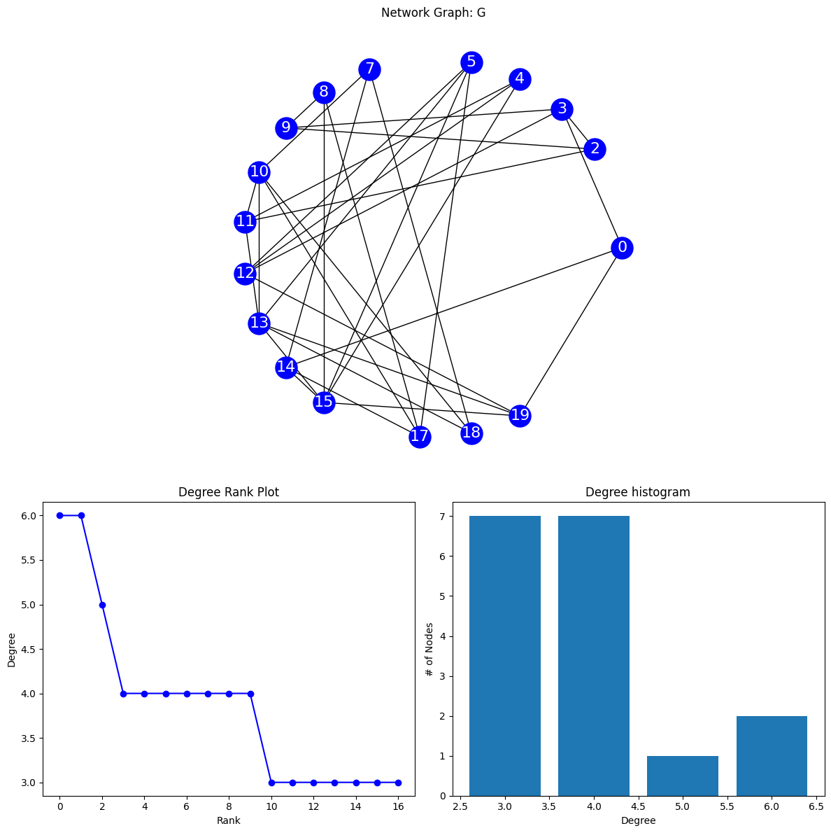
Gk=nx.k_core(G,2)print(Gk)draw_network(Gk)
Graph with 19 nodes and 37 edges
Code
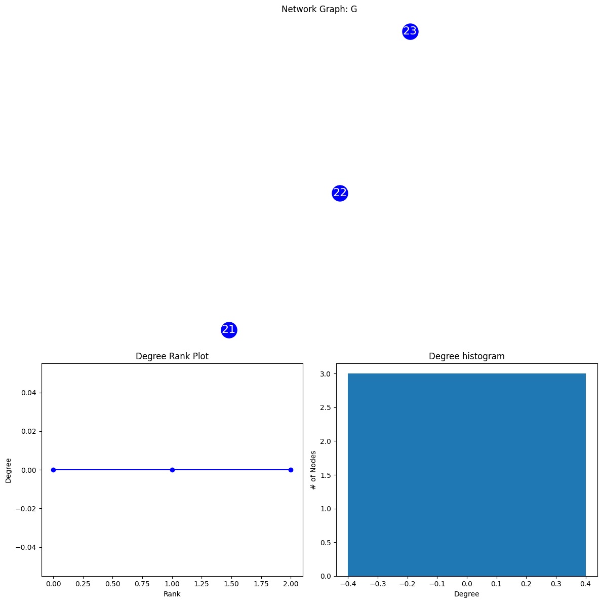
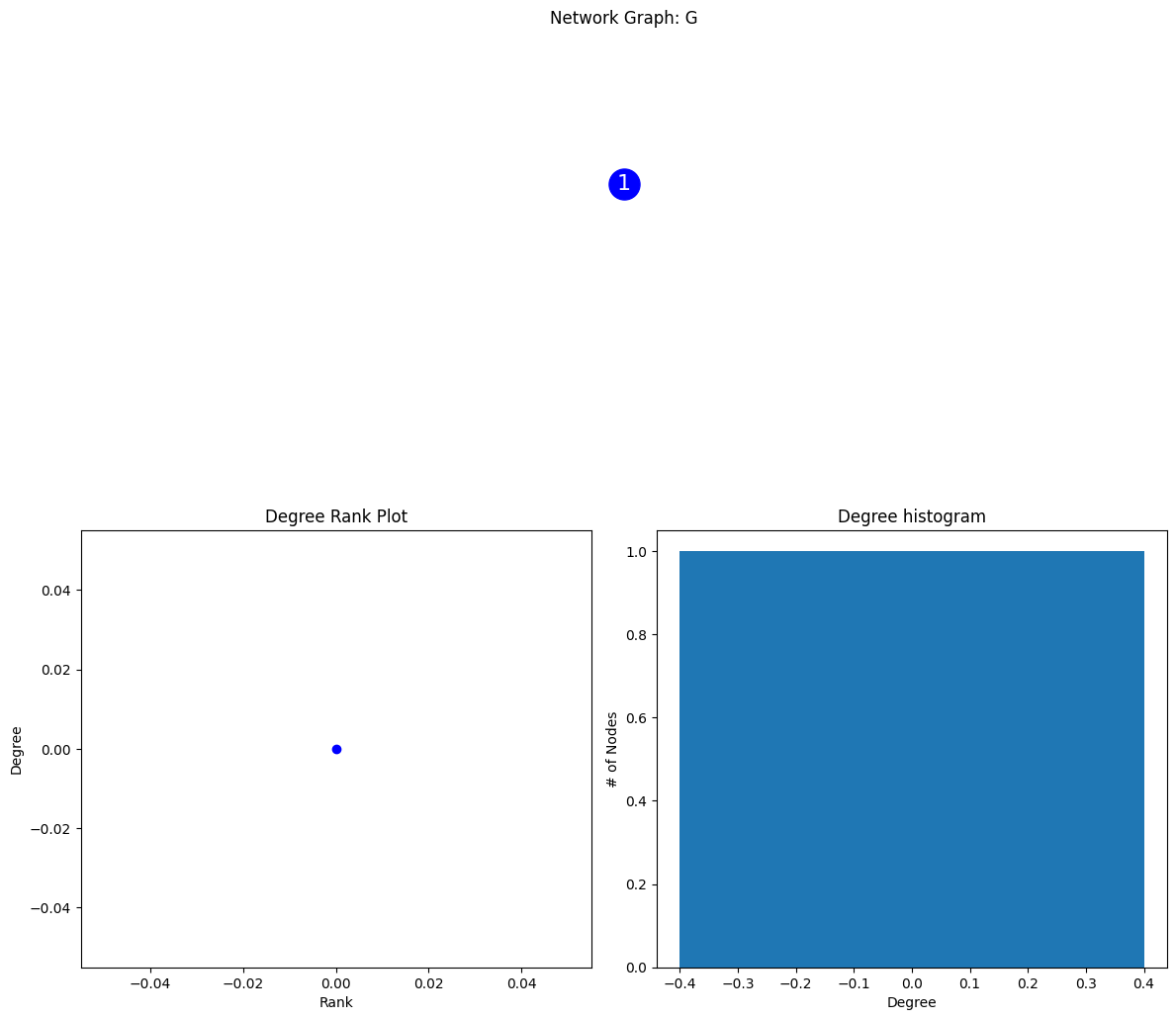
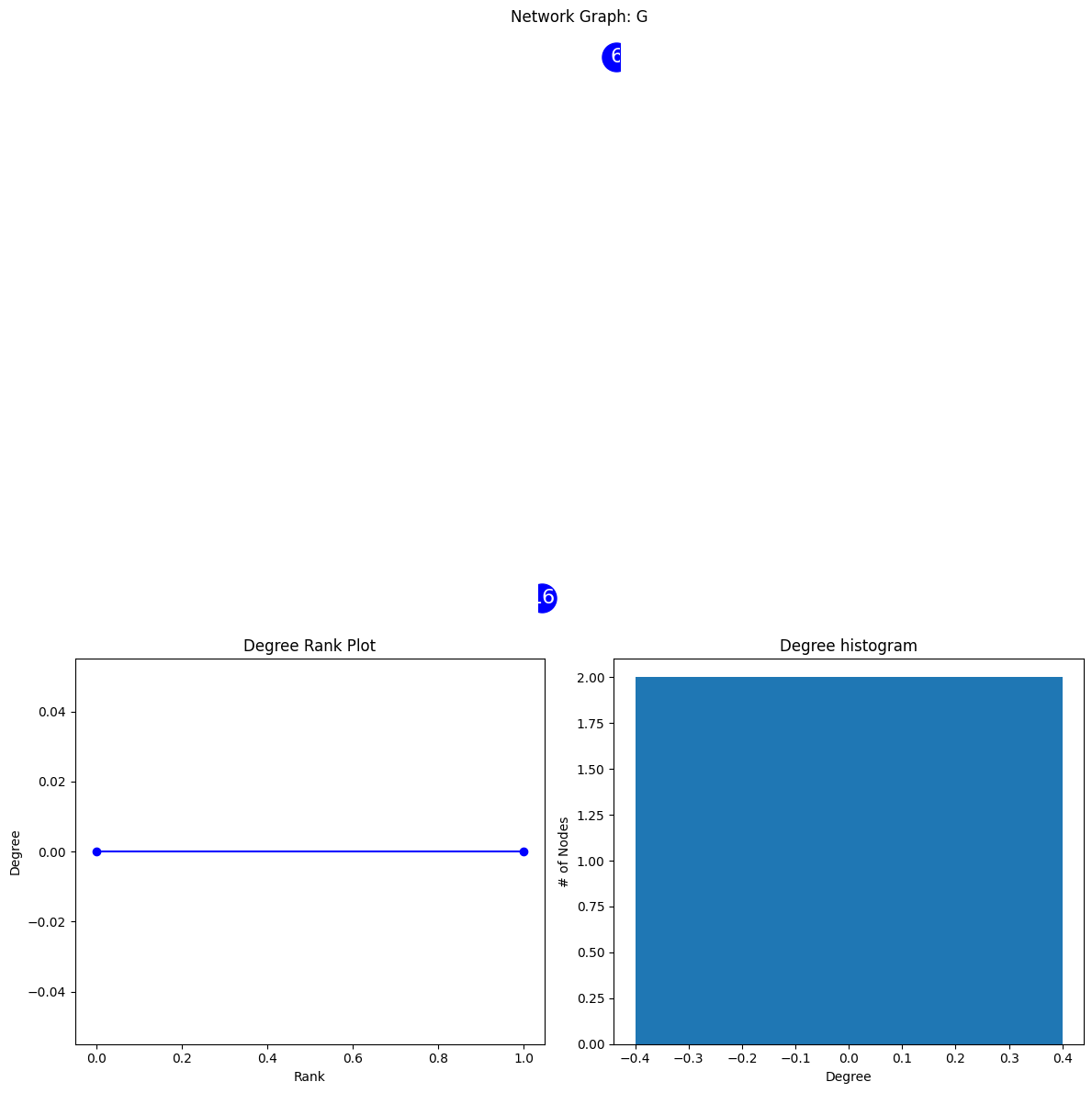
Gk=nx.k_shell(G,2)print(Gk)draw_network(Gk)
Graph with 2 nodes and 0 edges
Crust of K=2 shell
The crust in core-shell decomposition refers to the subset of nodes in a network that belong to the outermost layers or lower-order cores.
Nodes with the fewest connections
Found in the outer layers of the network
Less central and less influential
Compared to nodes in higher-order cores
Provides insight into the peripheral structure of the network
Important for understanding network disintegration and interactions of peripheral nodes
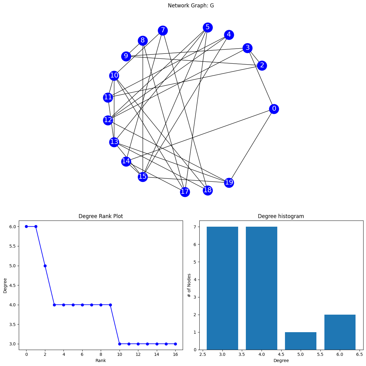
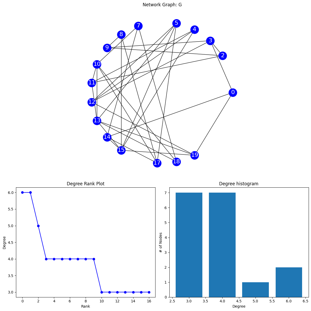
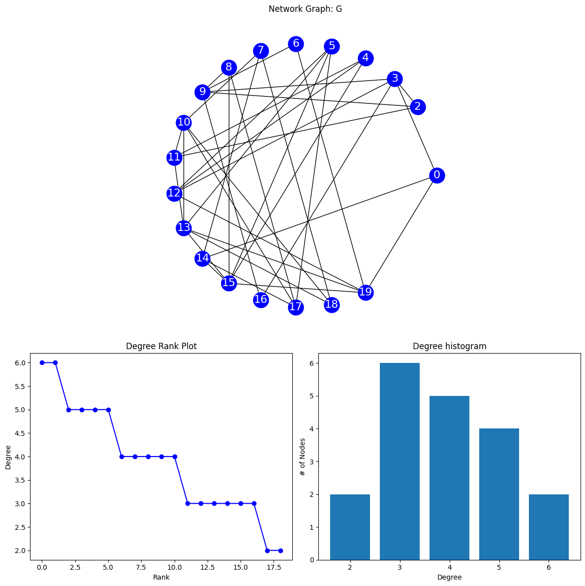
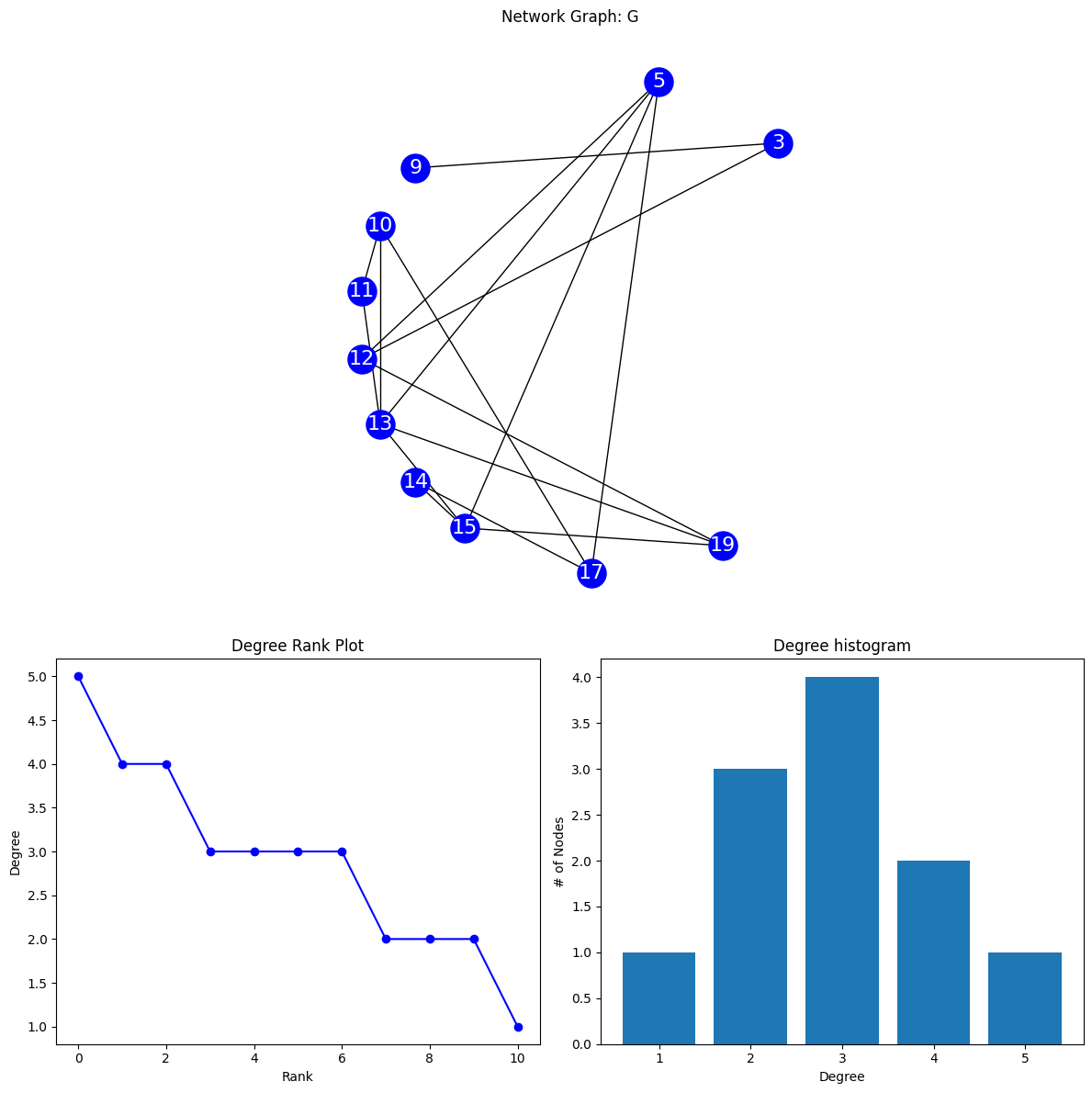
From the plots below, we can see that after k=3, removing nodes with 4 neighbors results in a graph where the degree of some remaining nodes is decreased by the removal.
This is why the code terminates when it does.
Removal condition appears to be that degree of nodes in remaining core is the same as the original network
Code
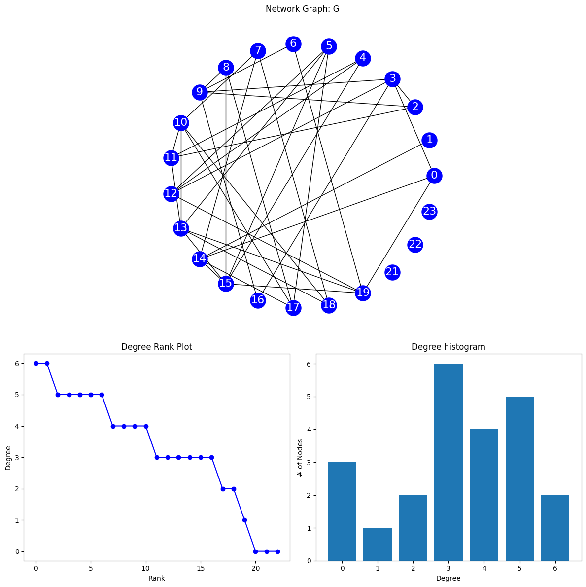
# original networkdraw_network(G)print(nx.degree(G))