Graph Laplacians Overview
Continous Laplacians
Background review
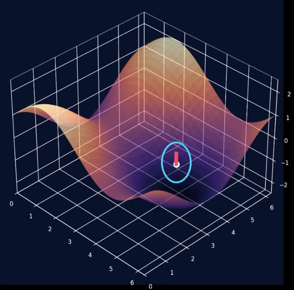
Recall: Common Differential Operators
In multivariable calculus, the two fundamental types of functions are:
- Scalar field: \(f(x, y, z)\)
- Vector field: \(\mathbf{F}(x, y, z) = \langle F_x, F_y, F_z \rangle\)
Here are the main differential operators that act on these fields:
- Gradient: \(\nabla f\) \(\rightarrow\) converts a scalar field into a vector field
- Divergence: \(\nabla \cdot \mathbf{F}\) \(\rightarrow\) converts a vector field into a scalar field
- Laplacian: \(\nabla^2 f = \nabla \cdot (\nabla f)\) \(\rightarrow\) operates on a scalar field, producing another scalar field
- Hessian: \(\operatorname{Hess} f = \nabla^2 f\) \(\rightarrow\) the matrix of second derivatives
- Curl: \(\nabla \times \mathbf{F}\) \(\rightarrow\) converts a vector field into a vector field
The Laplacian (Continuous case)
A scalar operator that takes a scalar field \(f(x_1,\dots,x_n)\) and reports, at each point, how much \(f\) differs from the average of its immediate surroundings.
\[\Delta f \;=\; \nabla\cdot\nabla f \;=\; \sum_{i=1}^{n}\frac{\partial^2 f}{\partial x_i^2} \;=\; \operatorname{tr}(\operatorname{Hess} f).\]
Reading the notation: \(\nabla\) is the gradient (a vector of first derivatives). Apply it twice, taking the divergence of the gradient, and the dot product collapses the vector back to a scalar, hence the “squared” in \(\nabla^2\). Three readings of the same object:
- Average vs. center (the key one): \(\Delta f(x_0) \propto \big(\text{average of } f \text{ on a tiny sphere around } x_0\big) - f(x_0)\).
- Divergence of the gradient: net outflow of the steepest-ascent field, so it pinpoints sources and sinks.
- Sum of curvatures: total concavity added up over every direction (the trace of the Hessian).
Sign: \(\Delta f > 0\) at a dip (center sits below its neighbors), \(\Delta f < 0\) at a bump, \(\Delta f = 0\) when \(f\) already equals its local average (harmonic).
In 3D Cartesian coordinates \((x, y, z)\) this is just the three unmixed second derivatives:
\[\nabla^2 f \;=\; \frac{\partial^2 f}{\partial x^2} + \frac{\partial^2 f}{\partial y^2} + \frac{\partial^2 f}{\partial z^2}.\]
In networks, discretize it and swap “tiny sphere” for “wired neighbors,” and \(\Delta\) becomes the graph Laplacian.
Intuition
Source: https://youtu.be/7ZmRqSeoylU?si=SKGiAa0eEAhCyVUv
Example: Diffusion/Heat Equation
\[\text { rate of change of } u=\kappa \text { (neighborhood average of } u-u \text { at the point). }\]
- Heat / diffusion equation: a field smooths out over time, flowing from high to low. \(\;\partial_t u = \kappa\,\nabla^2 u\)
- A hot spot bleeds warmth into its cooler surroundings until the temperature evens out, the way a drop of ink spreads through still water.
- What \(u\) is: the unknown scalar field \(u(\mathbf{x}, t)\), one number per point in space per moment in time, solved for from the equation.
- What it represents: whatever quantity is diffusing, named for the context.
- Literal heat: temperature, so \(u(\mathbf{x}, t)\) is the temperature at location \(\mathbf{x}\) and time \(t\).
- Other settings: chemical concentration, probability density, population, pressure, smoothed image intensity.
- Why “diffusion equation”: that same generality, one equation for any spreading quantity, is the reason for the alternate name.
Heat Equation on a Metal Sheet
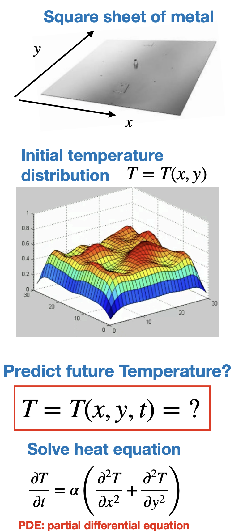
\[ \frac{\partial u}{\partial t} \;=\; \alpha\left(\frac{\partial^2 u}{\partial x^2} + \frac{\partial^2 u}{\partial y^2}\right) \;=\; \alpha\,\nabla^2 u. \]
- \(u(x, y, t)\): temperature at point \((x, y)\) on the sheet at time \(t\).
- \(\alpha = k/(\rho c_p)\): thermal diffusivity, how fast heat spreads (large for metals).
- \(\nabla^2 u\): the “neighborhood average minus center” reading. Cooler-than-surroundings warms, hotter cools.
To solve it you also need: - Initial: the starting temperature \(u(x, y, 0) = u_0(x, y)\) (say, a hot spot). - Boundary: edges held fixed (Dirichlet), insulated (Neumann), or losing heat to air (Robin).
Mesh the sheet into a grid of nodes and \(\alpha\nabla^2 u\) becomes \(-\alpha L u\): the graph diffusion from the deck.
Aside (optional): Solving the Heat Equation: Analytic vs Numerical
Analytic (separation of variables). Split \(u(x,t) = X(x)\,T(t)\), and the PDE breaks into two ODEs. The spatial part forces \(X\) to be an eigenfunction of \(\nabla^2\) (a sine/cosine mode set by the boundaries), and each mode decays in time at its own rate:
\[u(x,t) = \sum_k c_k\,\underbrace{\phi_k(x)}_{\text{spatial mode}}\;\underbrace{e^{-\alpha\lambda_k t}}_{\text{decay}}.\]
- Intuition: write the initial shape as a sum of modes (a Fourier series), then each mode just fades, the wiggliest (largest \(\lambda_k\)) fastest. Heat is a low-pass filter.
- Exact, but only for simple domains and boundaries.
Numerical (finite differences). Chop space into a grid and replace \(\nabla^2\) with the neighbor stencil, which is exactly \(-L\) on the grid graph. Then step time forward:
\[u^{n+1} = u^{n} + \alpha\,\Delta t\,(-L\,u^{n}).\]
- Intuition: at each tick, every node nudges toward the average of its neighbors. Repeat.
- Handles any shape and boundary, at the cost of grid resolution and a stability limit on \(\Delta t\).
Same skeleton. The analytic modes \(\phi_k\) are eigenvectors of the continuous \(\nabla^2\); the numerical update runs on eigenvectors of the discrete \(L\). Both say: decompose into modes, let each decay.
Additional Famous Equations Built on the Laplacian
- Laplace’s equation: equilibrium with no sources, the steady state everything relaxes to. \(\;\nabla^2 f = 0\)
- The shape a soap film or a stretched drumhead settles into: every point already sits at the average of its neighbors, so nothing pulls it anywhere.
- Poisson’s equation: equilibrium driven by a source \(\rho\) (charge, mass, heat). \(\;\nabla^2 \varphi = -\rho/\varepsilon_0\)
- Lay down charges and the potential field bends around them, dipping toward sources and rising near sinks, like a sheet weighed down wherever mass sits on it.
- Wave equation: disturbances oscillate and propagate at speed \(c\). \(\;\partial_{tt} u = c^2\,\nabla^2 u\)
- Pluck a string or strike a drum and the bump pushes on its neighbors, which push back, sending the ripple outward and letting it bounce.
- Helmholtz equation: the time-harmonic (single-frequency) modes of the wave equation. \(\;\nabla^2 f + k^2 f = 0\)
- The pure standing-wave patterns a system rings at, the fixed shapes behind a guitar note or the harmonics of a room.
- Schrödinger equation: quantum evolution, with \(-\nabla^2\) as the kinetic energy. \(\;i\hbar\,\partial_t \psi = -\tfrac{\hbar^2}{2m}\nabla^2\psi + V\psi\)
- A particle’s probability wave flows and interferes with itself, with sharper bends in the wave meaning more kinetic energy.
Graph Laplacians
For an undirected, unweighted graph with adjacency matrix \(A\) and degree matrix
Concepts generalize to weighted graphs with \(A\) and \(D\) replaced by \(W\) and \(D\)
The Graph Laplacian
For an undirected, unweighted graph with adjacency matrix \(A\) and degree matrix \(D = \operatorname{diag}(k_1, \dots, k_N)\) (degrees on the diagonal, zeros elsewhere):
\[L = D - A\]
- Diagonal entry \(L_{ii} = k_i\) (the degree of node \(i\)).
- Off-diagonal entry \(L_{ij} = -A_{ij}\) (a \(-1\) wherever an edge exists).
- Like \(A\), it is a square matrix that encodes the whole graph, but it carries far more usable spectral structure.
We will build it on this 4-node toy graph: a triangle \(\{0,1,2\}\) with a pendant node \(3\).
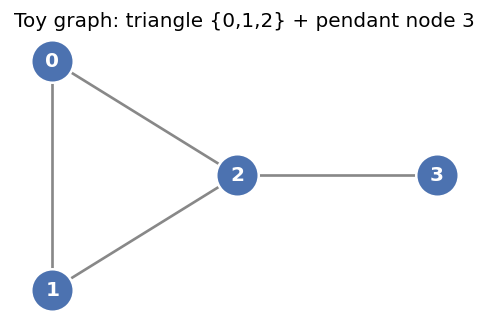
Building L by hand
Read the degrees straight off the picture: \(k_0 = 2,\ k_1 = 2,\ k_2 = 3,\ k_3 = 1\).
\[ A=\begin{pmatrix}0&1&1&0\\1&0&1&0\\1&1&0&1\\0&0&1&0\end{pmatrix},\quad D=\begin{pmatrix}2&0&0&0\\0&2&0&0\\0&0&3&0\\0&0&0&1\end{pmatrix},\quad L=D-A=\begin{pmatrix}2&-1&-1&0\\-1&2&-1&0\\-1&-1&3&-1\\0&0&-1&1\end{pmatrix} \]
Notice every row of \(L\) sums to zero. That single fact drives much of what follows.
Code for later calculations
Code
nodelist = [0, 1, 2, 3]
A = nx.to_numpy_array(G, nodelist=nodelist)
D = np.diag(A.sum(axis=1))
L = D - A

def show(M, name):
    print(f"{name} =")
    print(pd.DataFrame(M.astype(int), index=nodelist, columns=nodelist).to_string())
    print()

show(A, "A"); show(D, "D"); show(L, "L")
print("Row sums of L:", L.sum(axis=1).astype(int))   # all zero

fig, ax = plt.subplots(figsize=(4.0, 3.4))
im = ax.imshow(L, cmap="coolwarm", vmin=-3, vmax=3)
ax.set_xticks(range(4)); ax.set_yticks(range(4))
ax.set_xticklabels(nodelist); ax.set_yticklabels(nodelist)
for i in range(4):
    for j in range(4):
        ax.text(j, i, int(L[i, j]), ha="center", va="center",
                color="white" if abs(L[i, j]) > 1.5 else "black", fontweight="bold")
ax.set_title("L = D - A")
plt.colorbar(im, ax=ax, fraction=0.046, pad=0.04)
plt.show()
A =
0 1 2 3
0 0 1 1 0
1 1 0 1 0
2 1 1 0 1
3 0 0 1 0
D =
0 1 2 3
0 2 0 0 0
1 0 2 0 0
2 0 0 3 0
3 0 0 0 1
L =
0 1 2 3
0 2 -1 -1 0
1 -1 2 -1 0
2 -1 -1 3 -1
3 0 0 -1 1
Row sums of L: [0 0 0 0]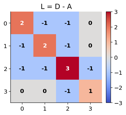
Moving from the Continuous Laplacian to the Graph Laplacian
Continuous Laplacian (Calculus)
For a smooth function \(f(x)\),
\[ \nabla^2 f = \frac{\partial^2 f}{\partial x^2} + \frac{\partial^2 f}{\partial y^2} +\cdots \]
- Measures how different a point is from its surroundings
- Large magnitude → rapid local change
- Zero → locally flat or in equilibrium
Graph Laplacian (Networks)
The graph Laplacian is the discrete version of the continuous Laplacian, it measures how much a node differs from its local neighborhood, just as the continuous Laplacian measures how a function differs from its local surroundings.
For a graph, the analogous quantity is
\[ (L\mathbf{x})_i = \sum_{j\in N(i)} (x_i-x_j), \]
where
\[ L = D - A. \]
- Compares a node’s value with its neighboring nodes
- Large value → node differs greatly from its neighbors
- Zero → node agrees with the average behavior of its neighborhood
The graph Laplacian \(L\) is an operator that maps a node signal \(x\) to the vector of local deviations, \((L x)_i=\sum_{j \sim i}\left(x_i-x_j\right)\), measuring how far each node’s value departs from its neighbors’.
Comparison
| Continuous Domain | Graph Domain |
|---|---|
| Space | Network |
| Nearby points | Neighboring nodes |
| Second derivative | Neighbor differences |
| \(\nabla^2\) | \(L=D-A\) |
Example: Demonstrating Graph Laplacian property
\[\boxed{(L x)_i=\sum_{j \in N(i)}\left(x_i-x_j\right)}\]
Graph: \(0-1-2\) (a path).
Signal: \(x=[0,4,0]\), so node 1 is a spike sitting above two flat neighbors.
Note: We can think of this square matrix as a linear operator that transforms a node-level vectors \(x\)
Right hand side
Apply the operator node by node using \((L x)_i=\sum_{j \in N(i)}\left(x_i-x_j\right)\) :
- Node 0 , neighbor \(\{1\}:(L x)_0=(0-4)=-4\)
- Node 1, neighbors \(\{0,2\}:(L x)_1=(4-0)+(4-0)=+8\)
- Node 2, neighbor \(\{1\}\) : \((L x)_2=(0-4)=-4\)
\[ L x=[-4,+8,-4] . \]
Left hand side
The adjacency \(A\) records who is wired to whom (the neighbor sets \(N(i)\) ), and the degree \(D\) is just its row sums on the diagonal:
\[ A=\left(\begin{array}{ccc} 0 & 1 & 0 \\ 1 & 0 & 1 \\ 0 & 1 & 0 \end{array}\right), \quad D=\left(\begin{array}{ccc} 1 & 0 & 0 \\ 0 & 2 & 0 \\ 0 & 0 & 1 \end{array}\right), \quad L=D-A=\left(\begin{array}{ccc} 1 & -1 & 0 \\ -1 & 2 & -1 \\ 0 & -1 & 1 \end{array}\right) . \]
Confirm with the matrix:
\[ L\left(\begin{array}{l} 0 \\ 4 \\ 0 \end{array}\right)=\left(\begin{array}{c} 1(0)-1(4)+0 \\ -1(0)+2(4)-1(0) \\ 0-1(4)+1(0) \end{array}\right)=\left(\begin{array}{c} -4 \\ 8 \\ -4 \end{array}\right) \]
Positive Semi-Definiteness
A symmetric matrix \(M\) is positive semi-definite (PSD) when
\[x^{T} M x \ge 0 \quad \text{for every vector } x.\]
- Intuition: it behaves like a multi-dimensional non-negative number. Applying it to a vector never flips that vector past \(90^\circ\).
- For an undirected graph \(L\) is symmetric, so its eigenvalues are real and its eigenvectors orthogonal.
- PSD then forces every eigenvalue to be non-negative:
\[0 = \lambda_1 \le \lambda_2 \le \dots \le \lambda_N.\]
From Node Deviations to the Quadratic Form
\[(L x)_i=\sum_{j \in N(i)}\left(x_i-x_j\right)\]
Weight each node’s deviation by its own value \(x_i\) and sum over all nodes:
\[x^{T} L x = \sum_i x_i\,(Lx)_i = \sum_i x_i \sum_{j \in N(i)}(x_i - x_j).\]
Every undirected edge \(\{i,j\}\) shows up twice, once from each endpoint. Add the pair:
\[x_i(x_i - x_j) + x_j(x_j - x_i) = (x_i - x_j)^2.\]
So the double sum collapses to one square per edge:
\[\boxed{\,x^{T} L x = \sum_{(i,j)\in E}(x_i - x_j)^2 \;\ge\; 0\,}\]
Example (\(x = [0,4,0]\) on the path, \(Lx = [-4, 8, -4]\)):
\[x^{T} L x = 0(-4) + 4(8) + 0(-4) = 32 = \underbrace{(0-4)^2}_{\text{edge }0\text{-}1} + \underbrace{(4-0)^2}_{\text{edge }1\text{-}2} = 32.\]
The operator \(L x\) reports per-node deviation;
the scalar \(x^{T} L x\) aggregates it into total disagreement across edges (the Dirichlet energy).
The Quadratic Form
The central identity:
\[x^{T} L x = \sum_{(i,j)\in E} A_{ij}\,(x_i - x_j)^2.\]
- Every term is a square, so the whole sum is \(\ge 0\). That is the proof that \(L\) is PSD.
- It measures how much a node signal \(x\) disagrees across edges.
- Take a \(0/1\) partition vector \(x\): each cut edge contributes exactly \(1\), each internal edge contributes \(0\). So \(x^{T} L x\) literally counts the cut edges.
Smoothness: Graph Dirichlet Energy
The same quantity \(x^{T} L x\) is the Dirichlet energy of the signal \(x\).
- Low energy means neighbors hold similar values: a smooth signal, homophily.
- High energy means the signal swings wildly across edges.
- Minimizing \(x^{T} L x\) subject to \(x \perp \mathbf{1}\) is exactly the relaxed RatioCut objective behind spectral clustering (more on this later).
Compare a smooth signal against a rough one on the toy graph.
Code
x_smooth = np.array([0.9, 1.0, 0.2, 0.0])   # similar on the triangle, decays on the pendant
x_rough  = np.array([1.0, 0.0, 1.0, 0.0])   # alternates, disagrees on most edges

for name, v in [("smooth", x_smooth), ("rough ", x_rough)]:
    print(f"{name} x = {v}   ->   Dirichlet energy  x^T L x = {v @ L @ v:.2f}")
smooth x = [0.9 1. 0.2 0. ] -> Dirichlet energy x^T L x = 1.18
rough x = [1. 0. 1. 0.] -> Dirichlet energy x^T L x = 3.00\(\lambda_1 = 0\) and the All-Ones Eigenvector
Because every row of \(L\) sums to zero,
\[L\mathbf{1} = \mathbf{0}, \qquad \mathbf{1} = [1, 1, \dots, 1]^{T}.\]
So \(\mathbf{1}\) is an eigenvector with eigenvalue \(0\), and the smallest eigenvalue is always exactly zero.
Multiplicity of 0 Counts Components
A sharper statement:
the number of zero eigenvalues equals the number of connected components.
- One component gives exactly one zero eigenvalue (the \(\mathbf{1}\) vector).
- \(k\) components give \(k\) zero eigenvalues. Each zero eigenvector is constant on its own component and zero elsewhere.
Edge case: two disjoint triangles, no bridge between them.
eigenvalues: [-0. -0. 3. 3. 3. 3.]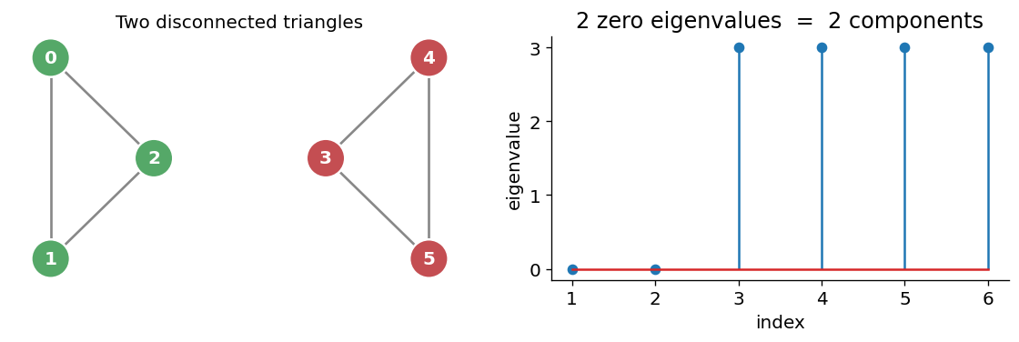
Algebraic Connectivity: the Fiedler Value \(\lambda_2\)
The second smallest eigenvalue \(\lambda_2\) is the algebraic connectivity, or Fiedler value. It grades how well-connected and how robust the graph is.
- \(\lambda_2 = 0\): the graph is disconnected.
- \(0 < \lambda_2 \ll 1\): a bottleneck or bridge, low resilience (a few edge removals split it).
- \(\lambda_2 = N\): achieved only by the complete graph \(K_N\), the densest possible.
So \(\lambda_2\) lives in \([0, N]\). Let us see all three regimes on \(N = 6\) nodes.
N = 6 for all three.  lambda_2 runs from ~0 up to N.
Path P6   : lambda_2 = 0.268
Barbell   : lambda_2 = 0.438
Complete  : lambda_2 = 6.000   (= N = 6, only K_N reaches this)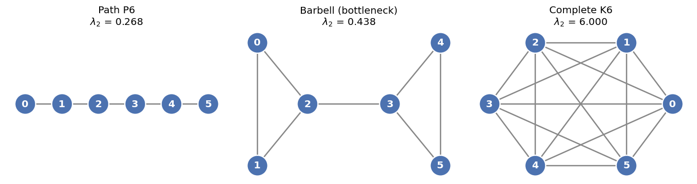
The Fiedler Vector Finds the Cut
The eigenvector belonging to \(\lambda_2\) is the Fiedler vector. It assigns each node a real number.
Spectral bisection: split nodes by the sign of their Fiedler value. The split lands across the bottleneck, cutting as few edges as possible.
On the barbell, this separates the two triangles and cuts only the single bridge.
Fiedler vector: [-0.465 -0.465 -0.261  0.261  0.465  0.465]
sign split    : [1 1 1 0 0 0]  (0 = green group, 1 = red group)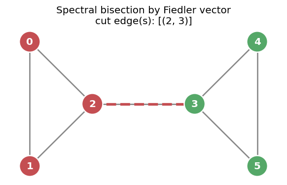
Why We Care
- Spectral clustering / community detection: eigenvectors of the smallest nonzero eigenvalues partition the graph with few cut edges.
- Connectivity and resilience: \(\lambda_2\) flags bottlenecks and fragile bridges before they fail.
- Diffusion and dynamics: \(L\) governs heat flow, consensus, synchronization, and spreading processes on the network.
- Embedding / dimension reduction: Laplacian Eigenmaps use \(L\)’s eigenvectors to place connected nodes near each other in a low-dimensional space.
Weighted Graphs
Almost nothing changes.
- Replace \(A\) with the weighted adjacency matrix, and put node strengths \(s_i = \sum_j A_{ij}\) on the diagonal: \(D = \operatorname{diag}(s_1, \dots, s_N)\).
- The edge-sum form now weights each disagreement:
\[x^{T} L x = \sum_{(i,j)\in E} A_{ij}\,(x_i - x_j)^2.\]
- Every property carries over unchanged in structure: PSD, the zero-eigenvalue / component link, and the Fiedler vector.
Directed Graphs: a Caveat
- For a directed graph \(A\) is asymmetric, so there is no single canonical Laplacian.
- The clean theory above (real eigenvalues, orthogonal eigenvectors, PSD) leans on symmetry.
- Several non-equivalent directed Laplacians exist (random-walk, magnetic, and others).
- Note discussed here
Detailed summary
The graph Laplacian is an important graph-level matrix similar to the adjacency matrix.
For an undirected, unweighted graph with adjacency matrix \(A\) and degree matrix \(D= \operatorname{diag}\left(k_1, \ldots, k_N\right)\) (node degree along the main diagonal an zero everywhere else), the graph Laplacian is \[ L=D-A \]
It is important because it is another well behaved, mathematically, well structured square matrix that describes the graph
One of the major reasons that it is important is that it is a positive semi-definite matrix which has several important properties in linear algebra.
Recall the definition of a positive semi-definite matrix.
A positive semi-definite matrix acts like a multi-dimensional “non-negative number,” meaning that when you use it to transform any vector, the resulting vector never points in the opposite direction of the original (the angle between them is always less than or equal to \(90^\circ\))
Mathematically, a symmetric matrix \(M\) is positive semi-definite if for every non-zero vector \(x\), the quadratic form is non-negative: \(x^T M x \ge 0\)
Motivation: Where it emerges in network science
- Community Detection & Spectral Clustering: The eigenvectors corresponding to the smallest non-zero eigenvalues of the Laplacian allow for optimal partitioning of a network into clusters or communities, minimizing the number of edges cut between groups.
- Network Connectivity & Resilience: The second smallest eigenvalue (\(\lambda_2\)), known as the algebraic connectivity or Fiedler value, quantifies how well-connected a network is and measures its robustness against node or edge failures.
- Interpretation of the Fiedler value
- \(\lambda_2=0\) (Disconnected): The network contains two or more components; global diffusion or communication between them is impossible. This is the \(\lambda_2\) instance of the general property that the multiplicity of eigenvalue 0 equals the number of connected components.
- \(0<\lambda_2 \ll 1\): The graph has a structural bottleneck or bridge, a relatively small edge cut separates it into two large pieces. This is the regime the Fiedler vector exploits for spectral bisection (it identifies where that bottleneck cut lies), but a small \(\lambda_2\) also signals low resilience: removing a small number of bridge edges disconnects the network.
- \(\lambda_2=N\) (Complete graph \(K_N\) ): This is the maximum value \(\lambda_2\) can take for any graph on \(N\) nodes, achieved uniquely by \(K_N\), reflecting maximal density: every node is directly connected to every other, so no edge cut can disconnect any part of the graph without removing nearly all of it.
- Interpretation of the Fiedler value
- Diffusion and Spreading Processes: The Laplacian governs continuous-time dynamical processes on networks, such as heat diffusion, consensus protocols, synchronization, and how information or diseases spread across nodes.
- Graph Embedding & Dimension Reduction: Techniques like Laplacian Eigenmaps use the matrix’s eigenvectors to map high-dimensional network data into lower-dimensional spaces while preserving the local geometric structure and distances between connected nodes.
Important properties: From a linear algebra perspective, the graph Laplacian matrix (\(L = D - A\)) possesses several elegant structural properties that make it a powerful tool for analysis:
Symmetry: For any undirected graph with real weights, \(L\) is a symmetric matrix (\(L = L^T\)). This guarantees that all of its eigenvalues are real numbers and its eigenvectors are orthogonal.
Positive Semi-Definiteness: The Laplacian is a positive semi-definite matrix (\(x^T L x \ge 0\) for any vector \(x\)). Consequently, all of its eigenvalues are non-negative (\(0 = \lambda_1 \le \lambda_2 \le \dots \le \lambda_n\)).
Trivial Smallest Eigenvalue: The smallest eigenvalue is always exactly zero (\(\lambda_1 = 0\)). Its corresponding eigenvector is the all-ones vector (\(\mathbf{1} = [1, 1, \dots, 1]^T\)), because each row of \(L\) sums to zero.
Multiplicity of Zero Indicates Components: The multiplicity of the eigenvalue \(0\) equals the exact number of connected components in the graph. For a fully connected graph, there is exactly one zero eigenvalue.
- The algebraic multiplicity of an eigenvalue refers to how many times it appears as a root of the matrix’s characteristic equation
Diagonally Dominant: \(L\) is a diagonally dominant matrix because the diagonal entry for any node \(i\) (its degree, \(D_{ii}\)) is exactly equal to the sum of the absolute values of the off-diagonal entries in that row (\(\sum_{j \neq i} |A_{ij}|\)).
Quadratic form: The quadratic form of the graph Laplacian \(L\) for a node state vector \(x \in \mathbb{R}^n\) is \(x^T L x\)
This can be written in two ways, depending on how the sum is constructed \(\quad x^T L x=\frac{1}{2} \sum_{i, j} A_{i j}\left(x_i-x_j\right)^2=\sum_{(i, j) \in E} A_{i j}\left(x_i-x_j\right)^2\) (where the 1/2 handles double counting in the summation)
Graph Dirichlet Energy: It quantifies the global smoothness of a graph signal \(x\). A low value indicates homophily, where structurally adjacent nodes share highly correlated states.
Spectral Clustering Objective: Minimizing this quadratic form under the constraint \(x \perp \mathbf{1}\) directly solves the relaxed RatioCut problem, partitioning the network into communities while minimizing inter-cluster edge cuts.
Weighted case
- Replace \(A\) with the weighted adjacency matrix, \(D = \text{diag}(s_1, \ldots, s_N)\) using strength instead of degree. The quadratic form becomes \(x^T L x = \sum_{(i,j) \in E} A_{ij}(x_i - x_j)^2\)
- Everything above (PSD, \(0\)-eigenvalue/component correspondence, Fiedler vector) carries over unchanged in structure.
Directed Case: For directed graphs there is no single canonical Laplacian, because \(A\) is asymmetric and the clean spectral theory above relies on symmetry.
Key details
- \(L = D - A\) is symmetric, positive semi-definite, and diagonally dominant.
- \(x^{T} L x = \sum_{(i,j)\in E}(x_i - x_j)^2\) measures signal smoothness, and counts cut edges for a \(0/1\) split.
- \(\lambda_1 = 0\) always, with eigenvector \(\mathbf{1}\). The multiplicity of \(0\) equals the number of connected components.
- \(\lambda_2\) (the Fiedler value) grades connectivity, and its eigenvector bisects the graph.