Breadth-first search algorithm
Example-1: Undirected case
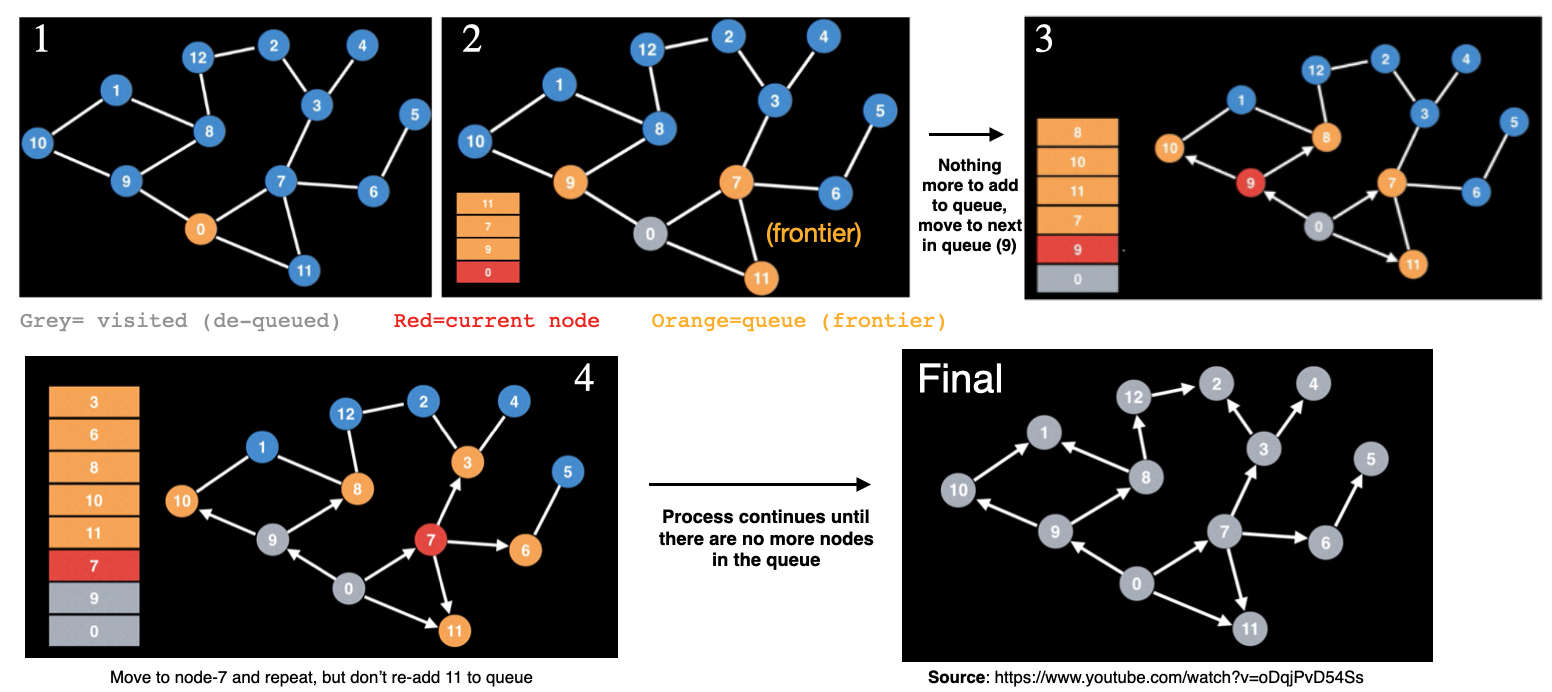
- Imagine trying to find a particular node satisfying some criterion, or just the path length
- A logical method is to start with a random node, then check neighbors, then check neighbors of neighbors, and so on.
- We use a
queueto keep track of the process (For more details see: https://www.youtube.com/watch?v=oDqjPvD54Ss )
Example-2: Undirected case
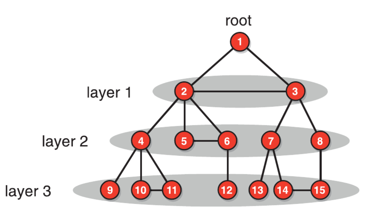
BFS naturally builds a tree by recording, for each node, which node discovered it (its “parent”), and because BFS processes nodes level by level, that parent relationship guarantees the path traced back from any node to the root through those parent pointers is the shortest possible path.
- Notice that the breadth-first search algorithm builds a directed
shortest-path tree - The tree maps the shortest paths between its root (the source node) and all other nodes.
- node-1 is selected as the source.
- visit the neighbors of node-1, which are 2 and 3. This is layer 1, including all nodes one step away from the source. We set the distance of those vertices from the source to one.
- Then we move to their neighbors 4,5,6,7,8, which are two steps away from the source (layer 2).
- Finally, we reach nodes 9,10,11,12,13,14,15, at distance three from the source (layer 3).
- Each layer contains all nodes having equal distance from the source.
- When completed, all nodes in the same connected component as the source have been assigned a distance from the source.
- To find the shortest path, we have to follow the links in the shortest-path tree backward from the target node through predecessors.
Source: DOI:10.1017/97811086539471
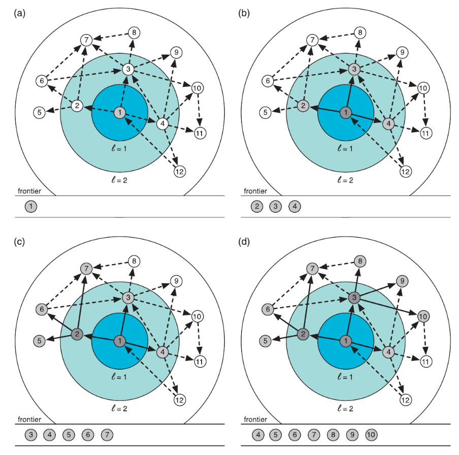
Example: Directed case
- The procedure is analogous for directed networks, except that we only reach nodes through directed paths from the source.1
What is DFS?
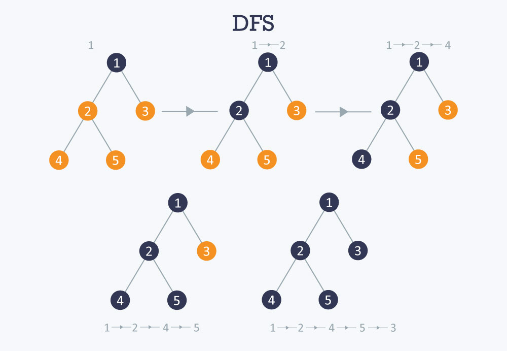
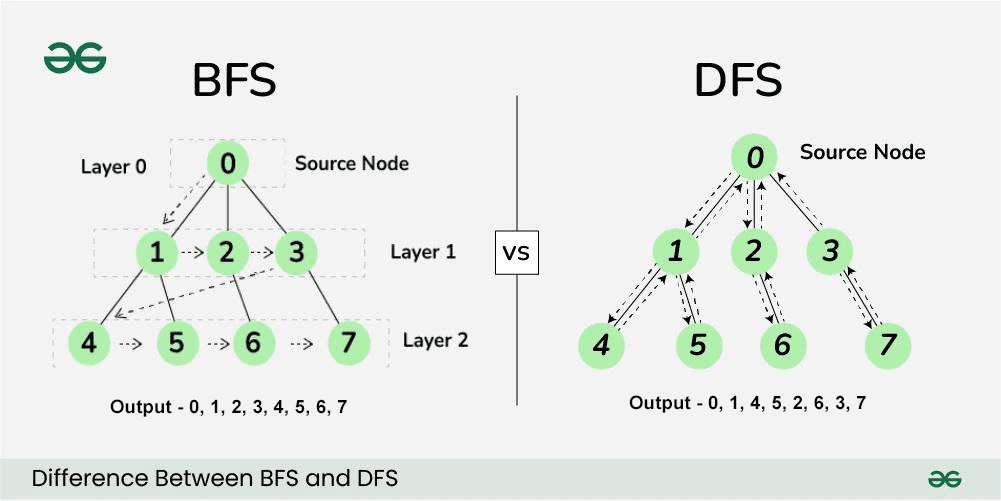
Unlike Breadth-First Search (BFS), which explores all neighbors at the current depth before moving to the next layer, Depth-First Search (DFS) explores as far as possible along each branch before backtracking.
- Depth-First Search (DFS) is a graph traversal algorithm that:
- Explores as far as possible along each branch before backtracking
- Mimics navigating a maze: pick a path, continue until a dead end, then backtrack to the last junction and try another route
Core Idea
Given a graph \(G = (V, E)\) and a starting node \(s\), DFS systematically visits every reachable node by always advancing to an unvisited neighbor before retreating.
The key data structure is a stack (either explicit, or implicitly via recursion).