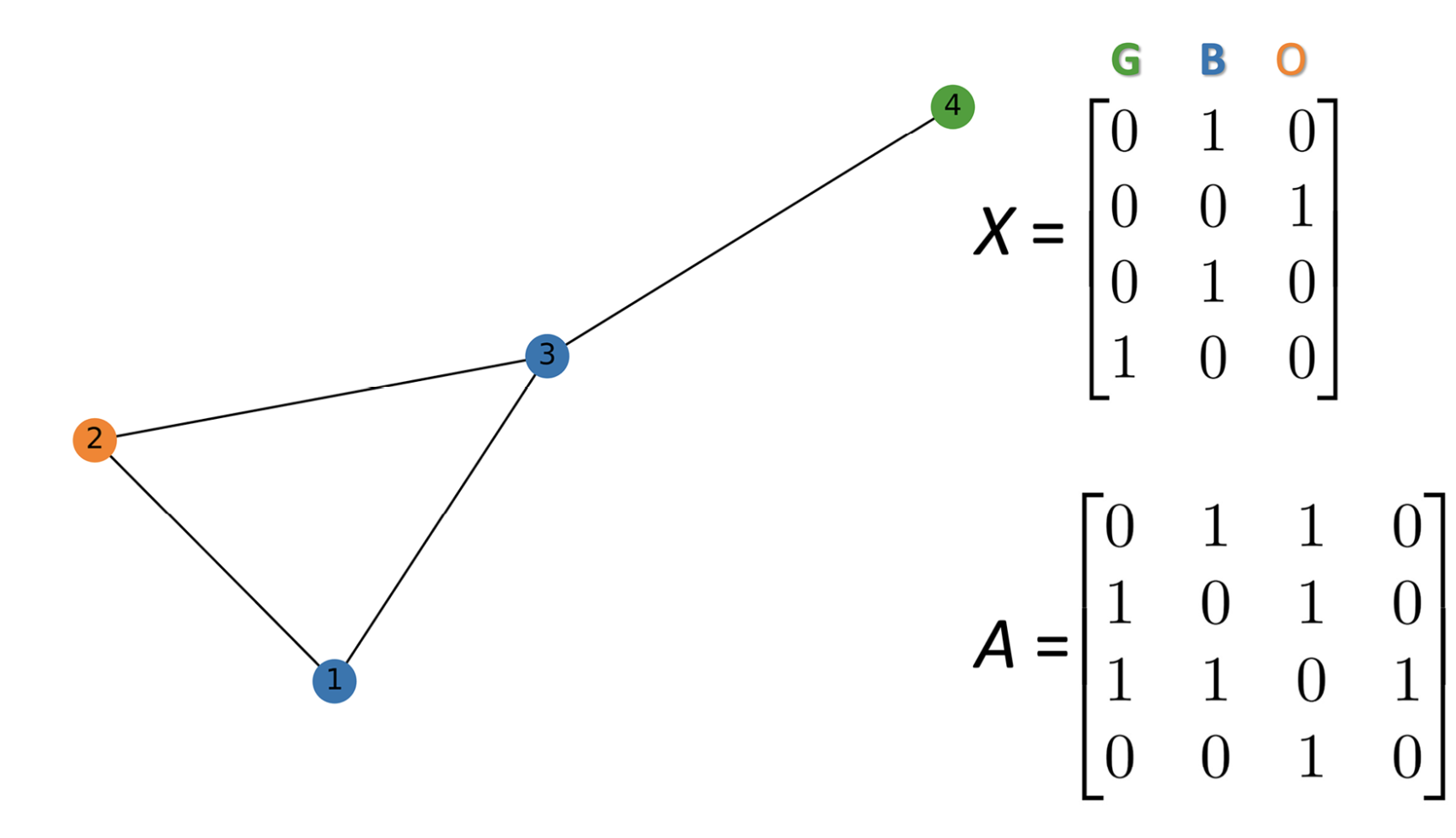
Adjacency matrix:
 [[0 1 1 0]
 [1 0 1 0]
 [1 1 0 1]
[0 0 1 0]]The GCN Architecture
Dataset
- Our playground shows a graph-level prediction task with small molecular graphs
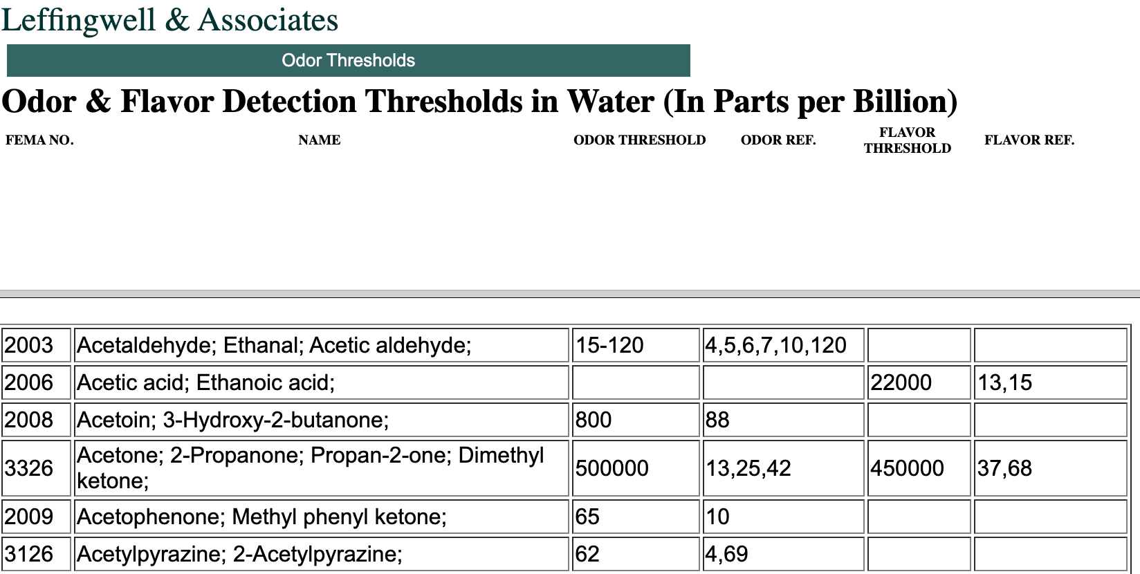
Leffingwell Odor Dataset: Composed of molecules with associated odor percepts (labels).- Predicting the relation of a molecular structure (graph) to its smell (target)
- Consider only a single binary label per molecule, classifying if a molecular graph smells “pungent” (e.g. garlic,peppermint, or mustard) or not
Data: Represent each molecule as a graph, atoms are nodes containing a one-hot encoding for atomic identity (Carbon, Nitrogen, Oxygen, Fluorine) and bonds are edges containing a bond type one-hot encoding (single, double, triple or aromatic).
Results
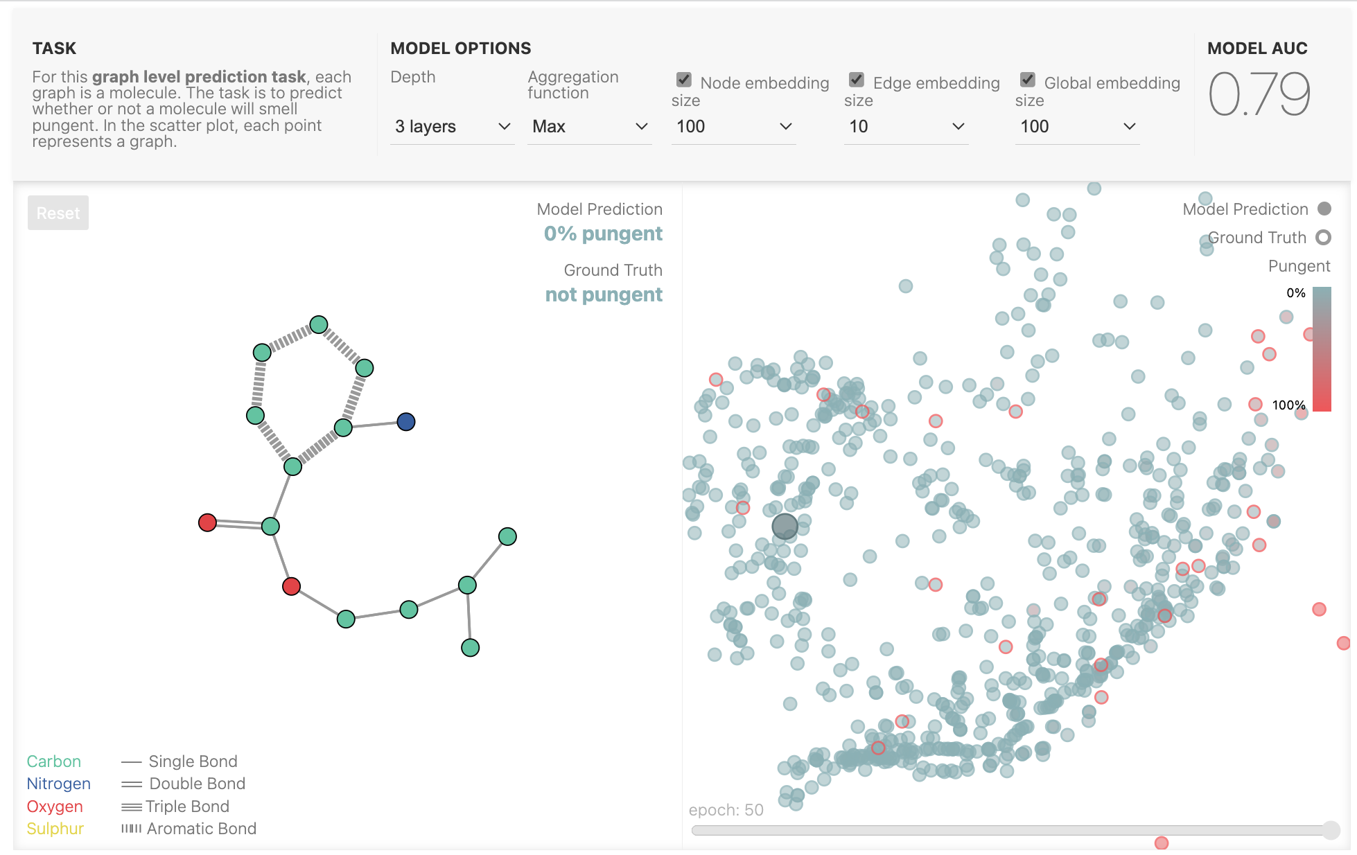
For this graph level prediction task, each graph is a molecule. The task is to predict whether or not a molecule will smell pungent. In the scatter plot, each point represents a graph.
You can edit the molecule to see how the prediction changes, or change the model params to load a different model.
Select a different molecule in the scatter plot.
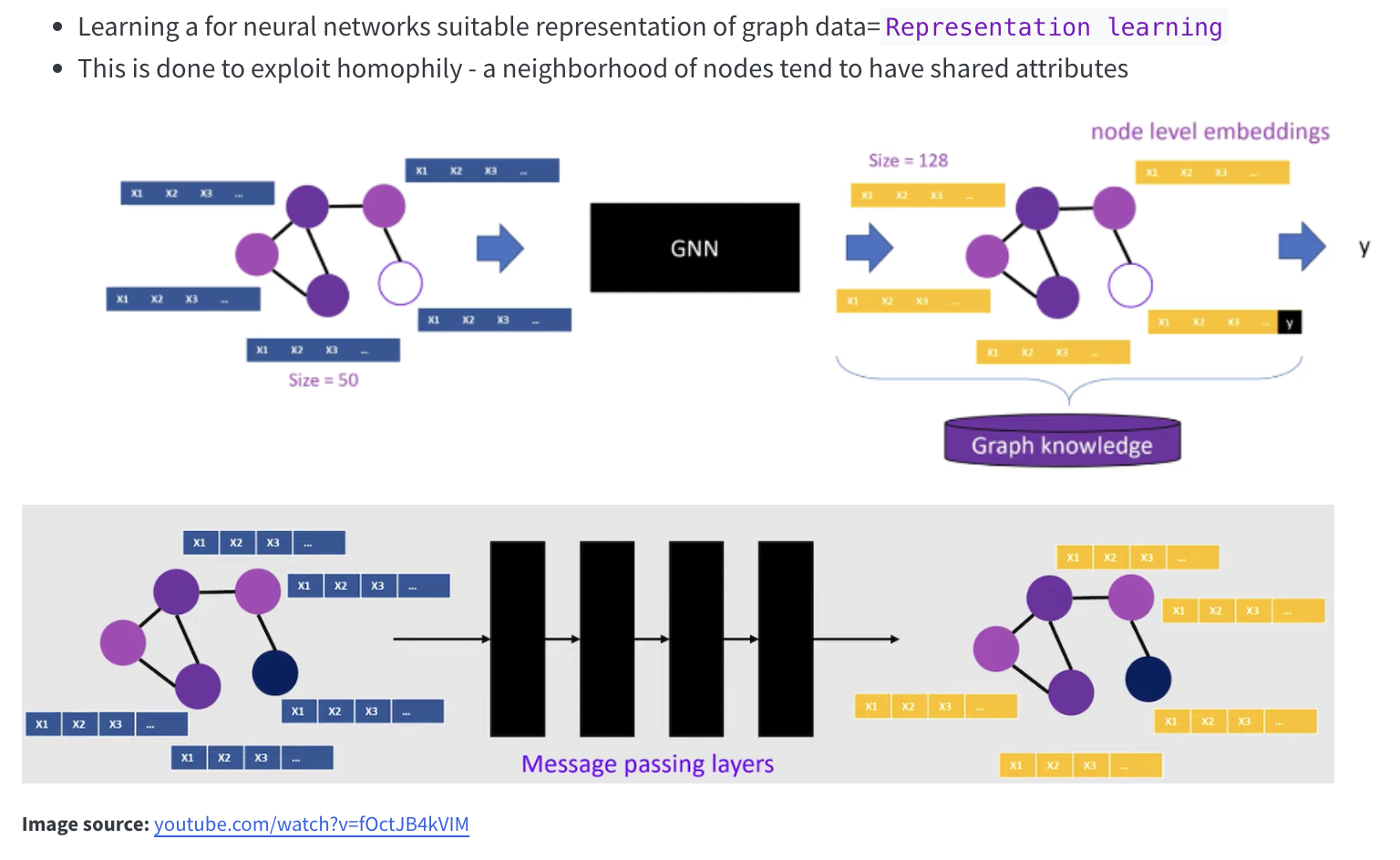
General idea
Weight Sharing: The CNN Analogy
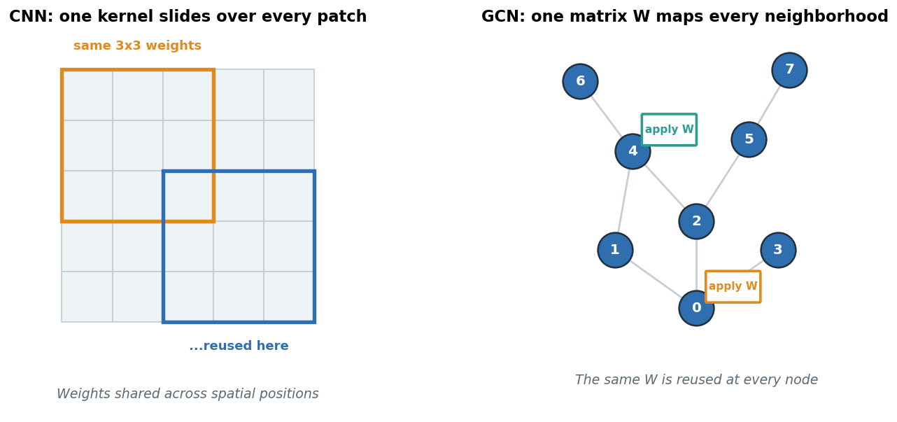
- CNN: one small kernel slides across an image: the same weights reused at every position.
- GCN: one matrix
Wis applied at every node’s neighborhood: the same weights everywhere. - Why it’s powerful:
- Few parameters: model size is independent of how many nodes/pixels there are.
- Generalizes: a pattern learned in one region works in another.
- Permutation-equivariant: relabeling nodes just relabels outputs; the graph has no fixed “first” node.
The mental model of a GCN
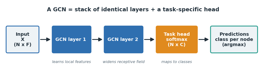
- A Graph Convolutional Network (GCN) is just a stack of identical layers plus a small task head.
- Each layer does one thing: mix each node with its neighbors, then re-express the result.
- We already know the single-layer rule: today we zoom out to the whole network.
- By the end you should see a GCN the way you see a CNN: a module you drop into a pipeline.
The full assembly line:
Here we use node level classification as an example, but below we will see how this pipeline can be used for different learning tasks.
Three steps, applied to every node
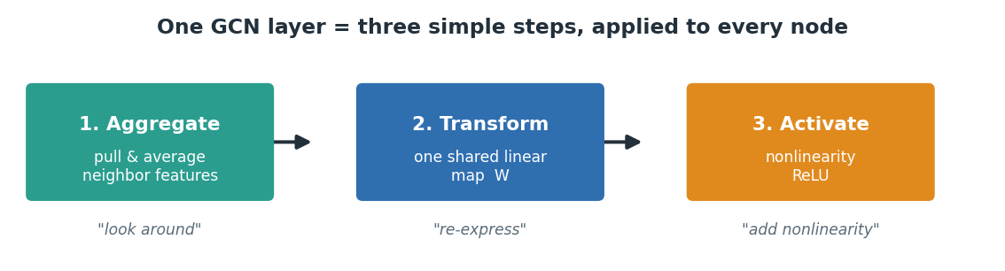
A single layer is the composition of three familiar operations:
- Aggregate: each node pulls in and averages its neighbors’ feature vectors (normalized).
- Transform: multiply by one shared weight matrix
W(a linear re-expression). - Activate: apply a nonlinearity like
ReLU(so stacked layers aren’t just one big linear map).
That’s the whole layer. Everything else is bookkeeping.
Stacking Layers = a \(k\)-Hop Receptive Field
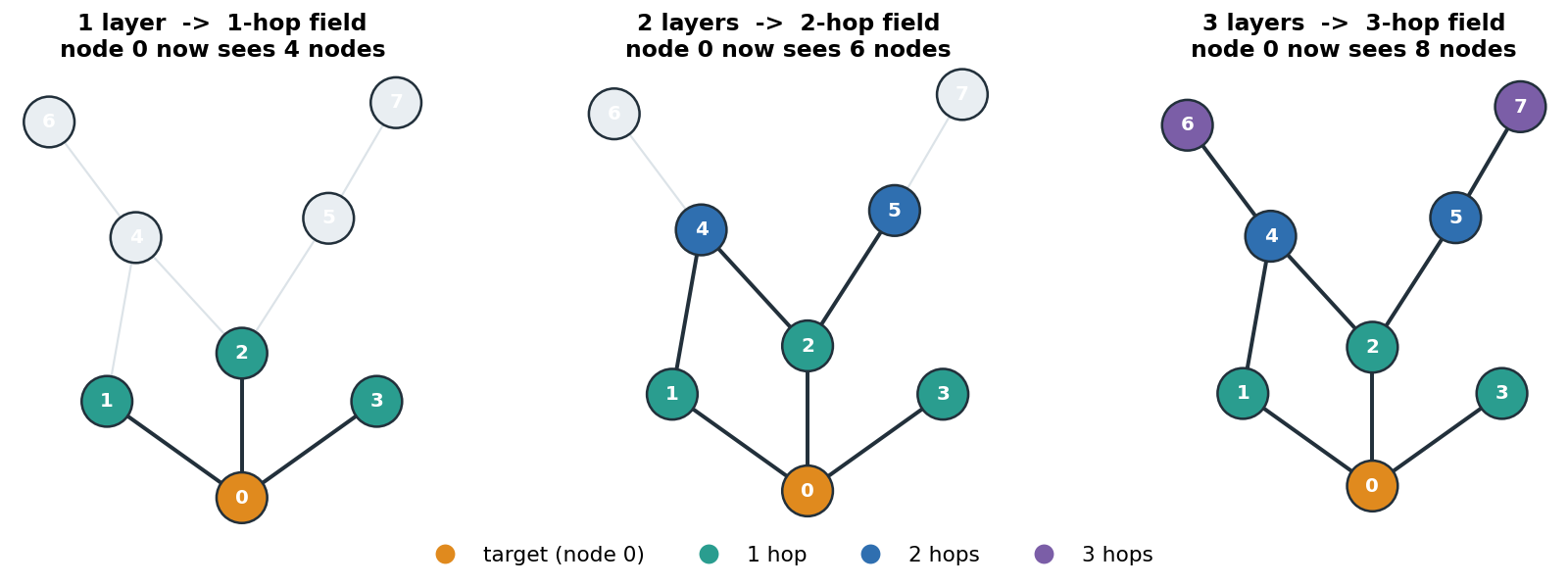
- One layer sees one hop: so we stack them
- 1 layer: a node blends with its direct neighbors → info travels 1 hop.
- 2 layers: neighbors have already blended with their neighbors → info travels 2 hops.
- \(k\) layers → each node’s output depends on everything within \(k\) hops: its \(k\)-hop receptive field.
- Same principle as a CNN: deeper = wider field of view, just measured in graph hops not pixels.
Alternative visualization
Data: Graph representation
- Undirected graph with \(n\) nodes and \(n \times n\) adjacency matrix \(\boldsymbol{A}\)
- \(n \times f_{\text {in }}\) node feature matrix \(\boldsymbol{X}\)
- Only feature is a one-hot representation of each node’s color-green (G), blue (B), or orange (O).
Visualize the graph
Node feature matrix:
 [[0. 1. 0.]
 [0. 0. 1.]
 [0. 1. 0.]
 [1. 0. 0.]]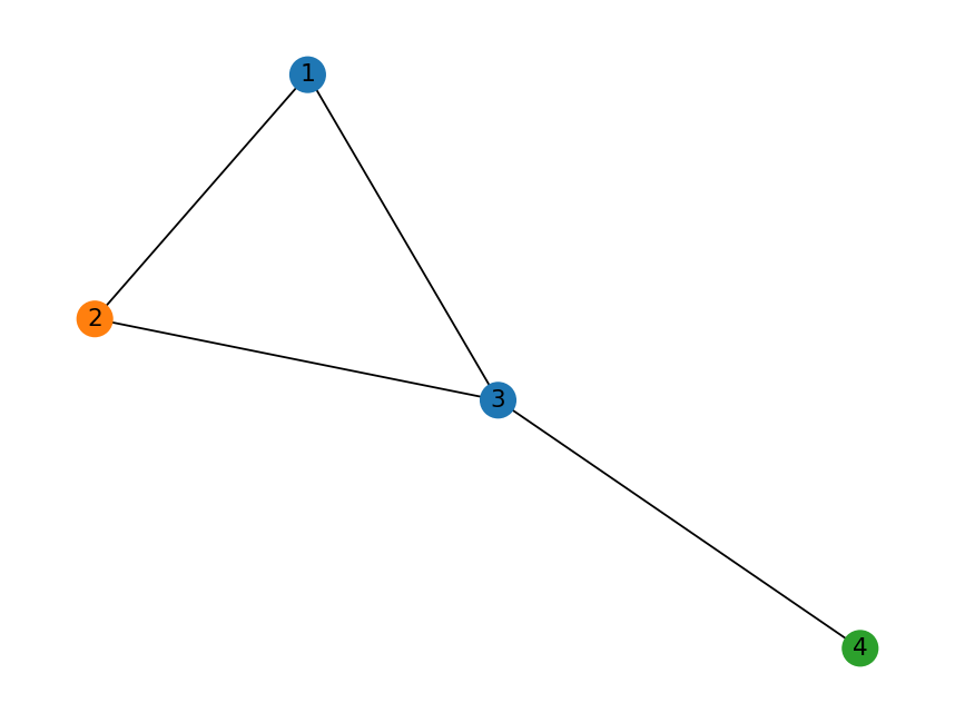
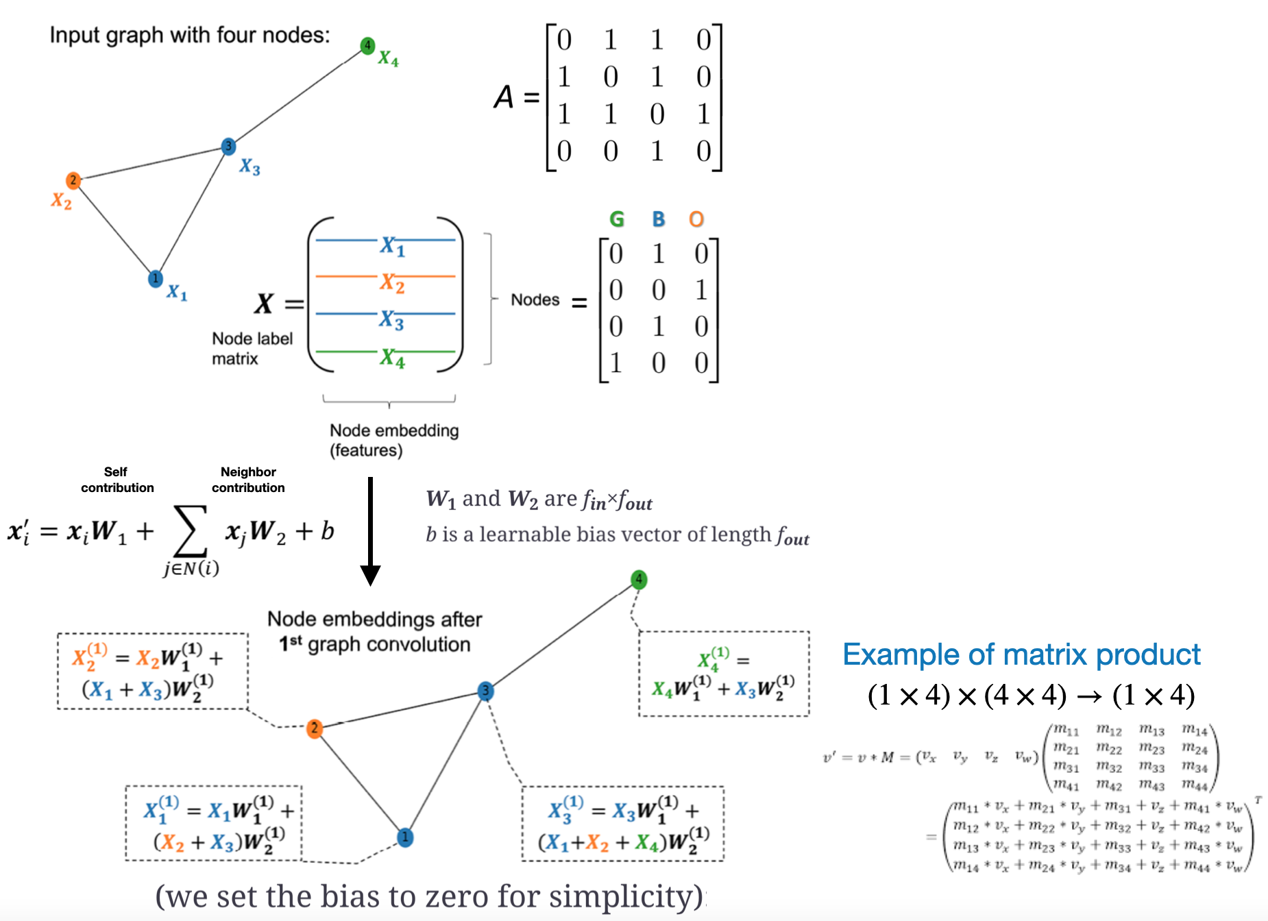
Graph convolution
- A single convolution is insufficient to capture a relationship between a node and another node located many edges away.
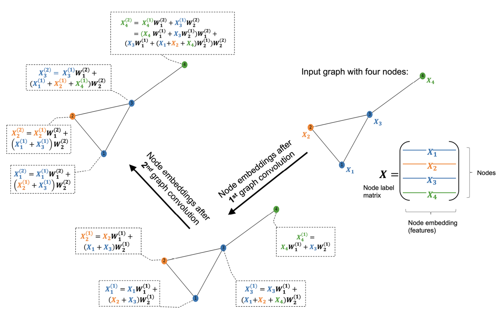
Multiple convolutional layers
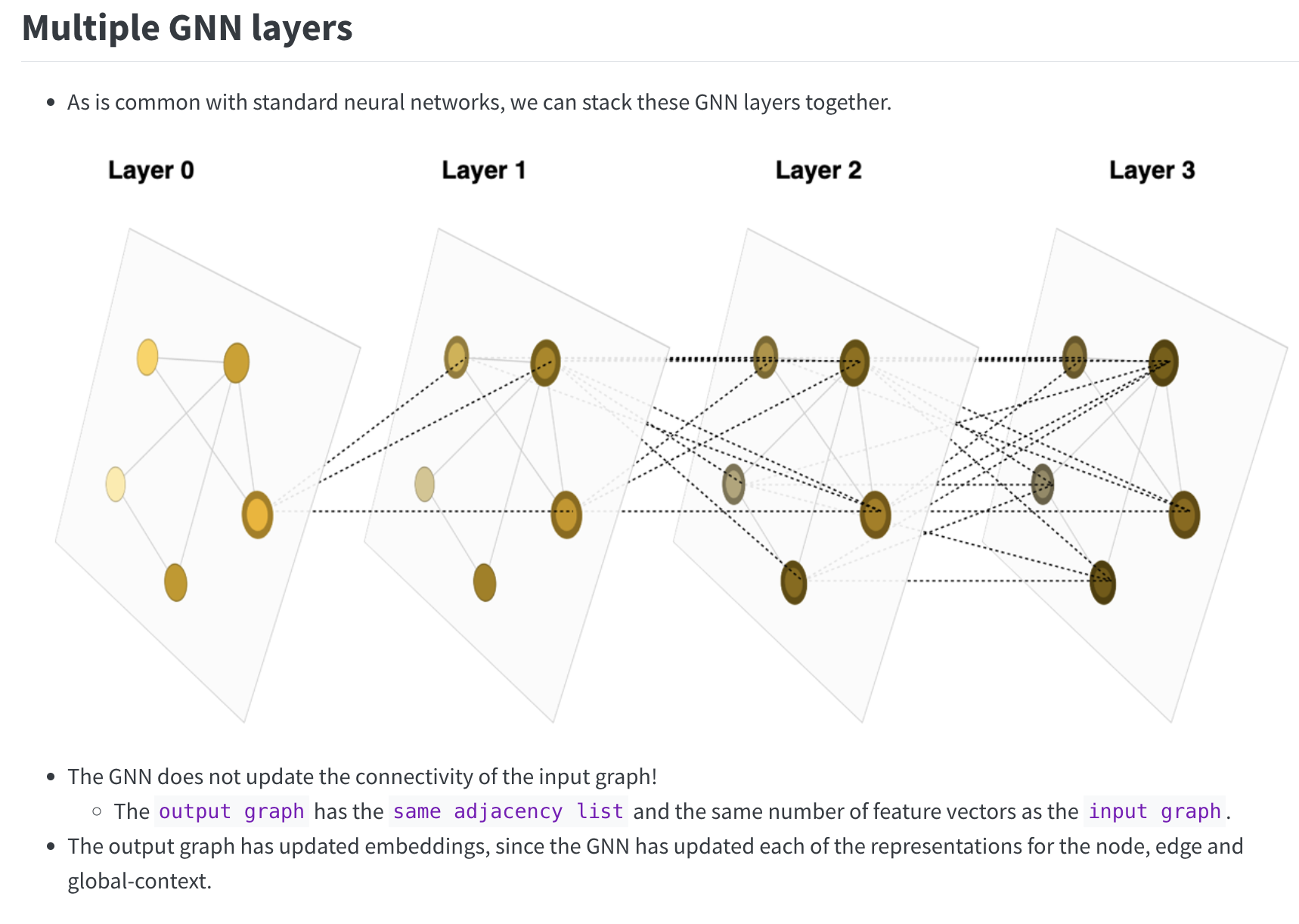
- We can stack multiple convolutions to capture more distant relationships in the network
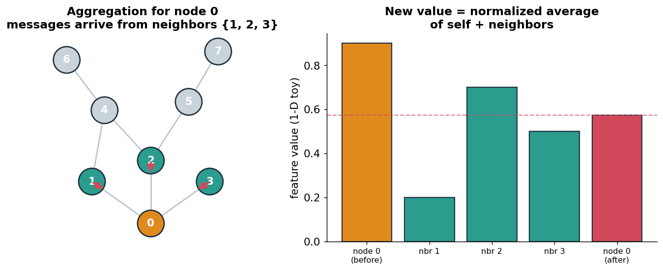
Step 1: Normalized neighbor aggregation
- Each node’s new value is a weighted average of itself + its neighbors.
- “Normalized” = we divide out node degrees so high-degree nodes don’t dominate (next section).
- Intuition: “describe me by the company I keep.”
- Left: messages flow into node 0 from
{1, 2, 3}. Right: the values get blended.
The Renormalization Trick: Building \(\hat{A}\)
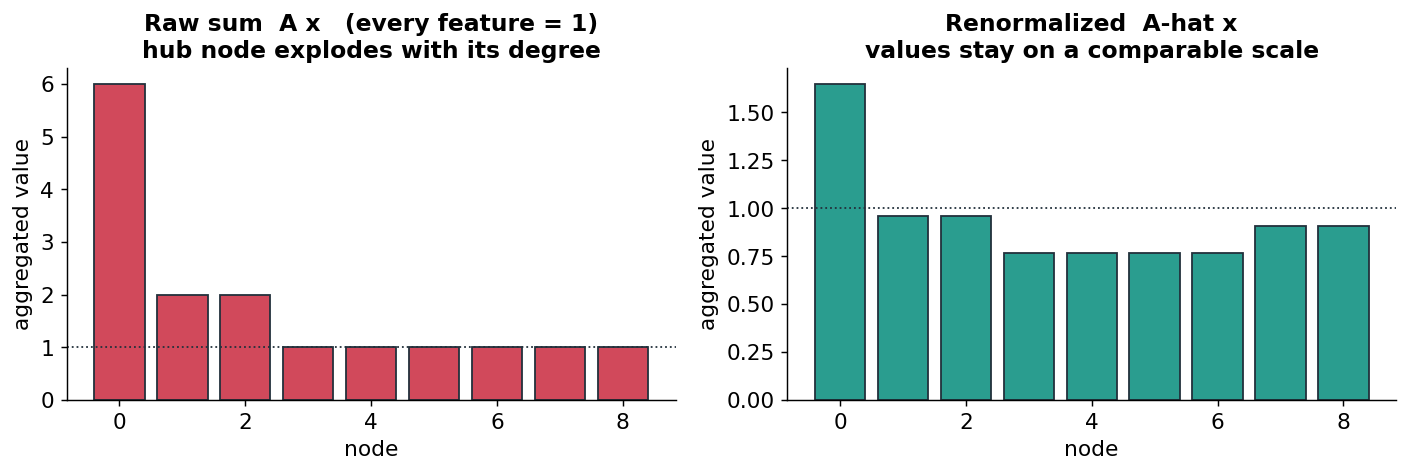
Why raw aggregation breaks
- Naive aggregation = “sum my neighbors’ features,” i.e. multiply features by
A. - Problem: a node with many neighbors gets a huge sum; a node with few gets a tiny one.
- Feature magnitudes then track degree, not content: and they can explode across layers.
- Below: one toy graph, every node’s feature = 1. Raw
A·xblows up at the hub;·xstays tame.
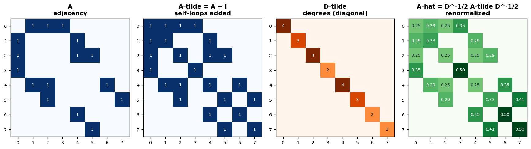
From \(A\) to \(\hat{A}\) in three moves
\[\hat{A} = \tilde{D}^{-1/2}\,(A+I)\,\tilde{D}^{-1/2}, \qquad \tilde{A}=A+I\]
- Add self-loops (\(A+I\)): a node should include its own features, not just neighbors’.
- Build \(\tilde D\): the diagonal degree matrix of \(\tilde A\) (each node’s neighbor count, +1 for itself).
- Symmetric normalize (\(\tilde D^{-1/2}\,\tilde A\,\tilde D^{-1/2}\)): scale each edge by both endpoints’ degrees.
Watch the four matrices for our 8-node graph:
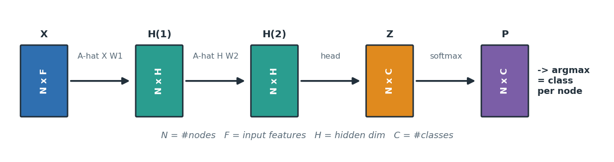
Dimensions flowing through the network
- Track the shapes and the whole model becomes obvious bookkeeping:
X: N × F (nodes × input features)- after layer 1: N × H (H = hidden width, your choice)
- after layer 2: N × H
- logits
Z: N × C (C = number of classes) - probabilities
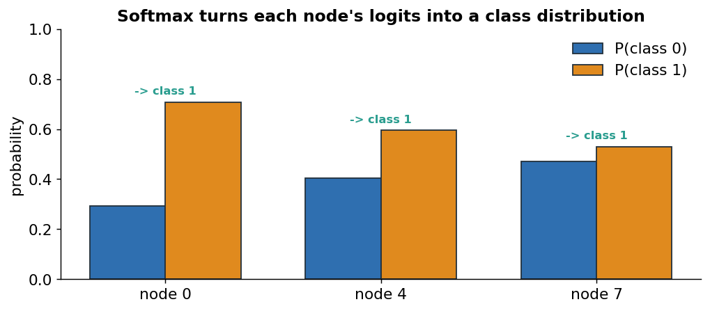
P: N × C, then argmax → one class per node.
The task head: softmax over node classes
- For node classification, the head is a softmax over the
Clogits of each node. - Output = a probability distribution per node; argmax picks the predicted class.
- Training minimizes cross-entropy on the labeled nodes; gradients flow back into every
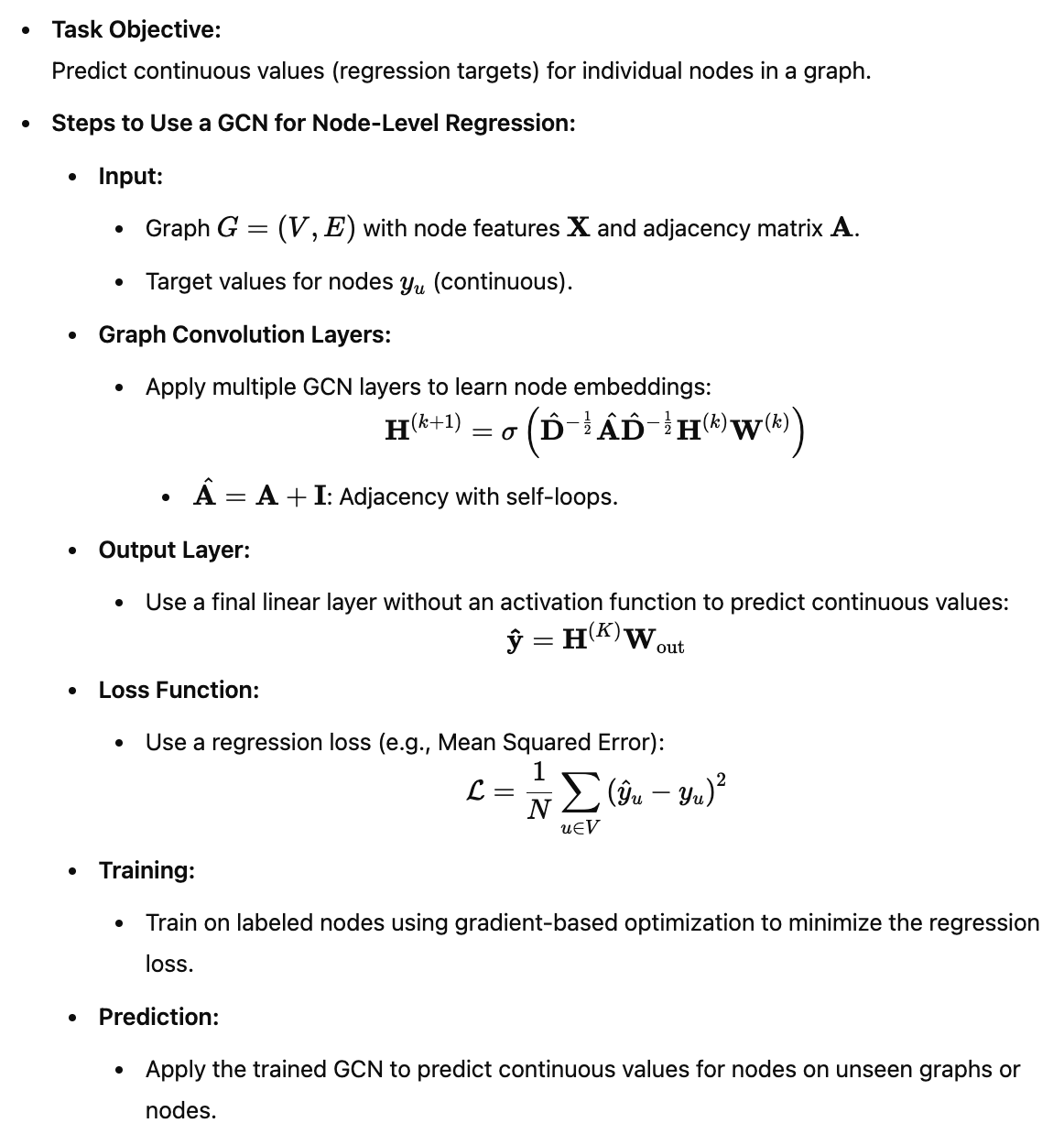
W. - Swap the head to change the task (graph-level readout, link scoring, regression, …).
How Deep Should You Go?
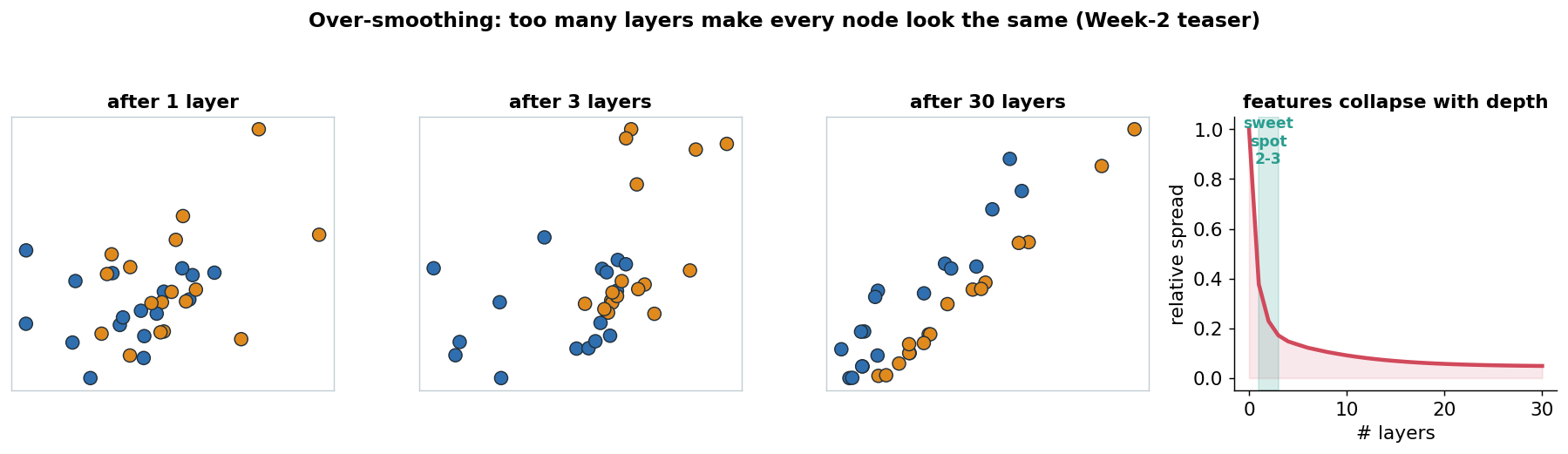
The 2–3 layer rule & over-smoothing
- Deeper GCNs repeatedly average node features: so they slowly become identical.
- Past a few layers, every node’s vector converges toward the same thing → over-smoothing.
- Classes stop being separable, and accuracy drops. The practical sweet spot is 2–3 layers.
- Below (Zachary’s karate club): two communities stay separated early, then collapse by depth 30.
Node-Level Tasks
Each node is processed independently after message passing.
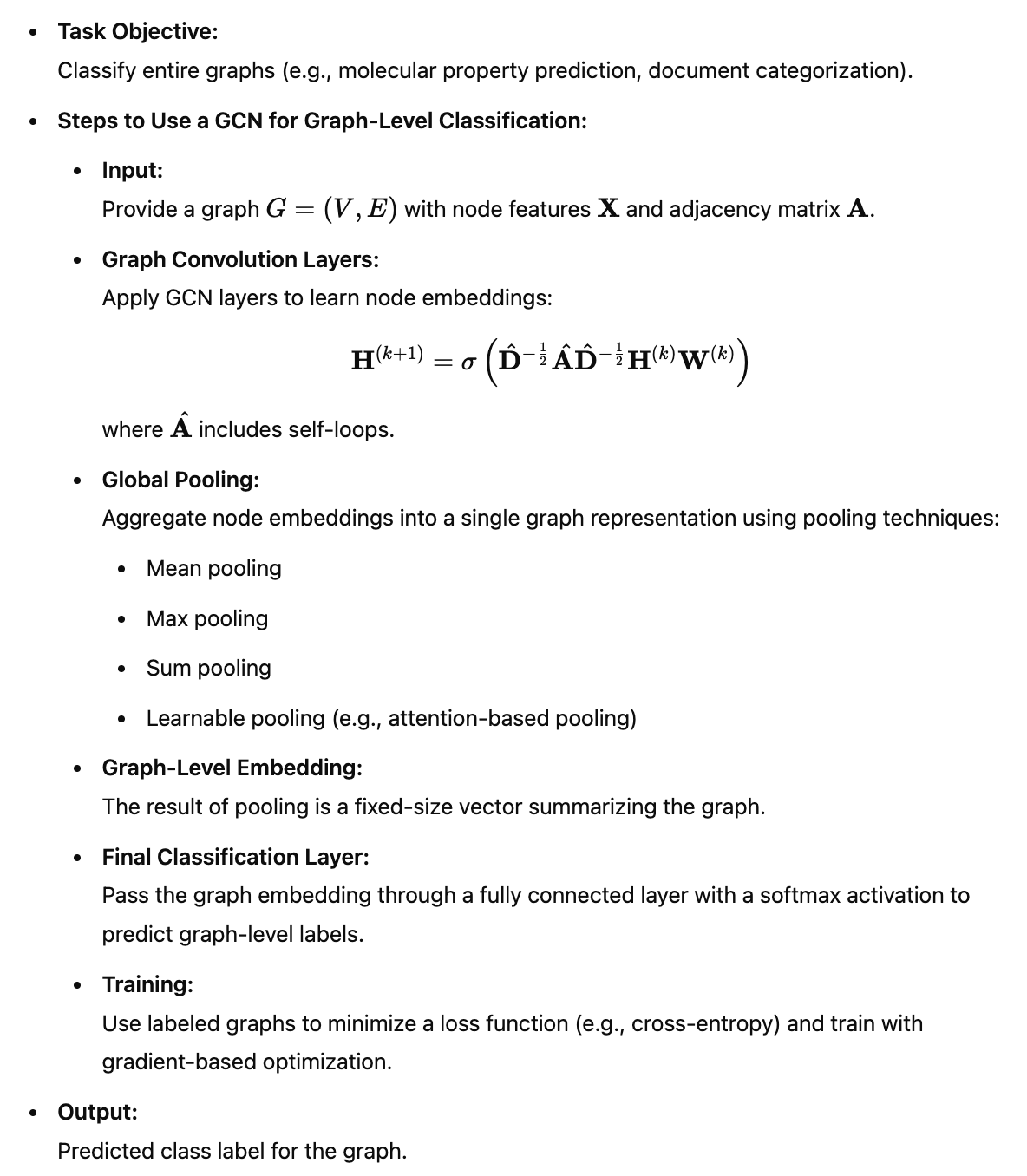
Graph-Level Tasks
All Node Embeddings
(h₁, h₂, ..., hₙ)
        │
        ▼
 Global Pooling
(mean / sum / max / attention)
        │
        ▼
 Graph Embedding
        │
        ▼
 Fully Connected Layer
        │
        ▼
 Prediction
The node embeddings are aggregated into a single graph representation before making a prediction.
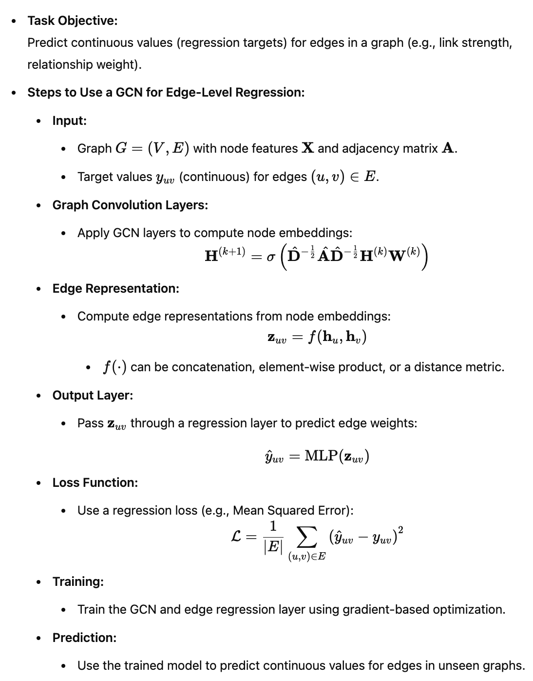
Edge-Level Tasks
Node Embedding hᵢ      Node Embedding hⱼ
        │                     │
        └──── Combine ─────────┘
      (concat, dot product,
        element-wise product)
               │
               ▼
      Fully Connected Layer
               │
               ▼
          Prediction
Predictions are made using the embeddings of the two nodes that define the edge.
Sources
This content is drawn primarily from the following sources:
- Machine Learning with PyTorch and Scikit-Learn: Develop Machine Learning and Deep Learning Models with Python Book by Liu Yuxi, Sebastian Raschka, and Vahid Mirjalili
- “A Gentle Introduction to Graph Neural Networks” https://distill.pub/2021/gnn-intro/
- “Graph neural network” https://en.wikipedia.org/wiki/Graph_neural_network
- Machine Learning with PyTorch and Scikit-Learn by Sebastian Raschka, Yuxi Liu, Vahid Mirjalili
- GPT-3.5 and GPT-4