3Blue1Brown, Essence of Linear Algebra: A staple resource for building geometric intuition, covering vectors, span and basis, linear transformations, determinants, column and null space, dot products, change of basis, and eigenvectors and eigenvalues. The playlist is roughly 16 short videos that give you a strong visual grasp of what each operation actually does.
Strength: Visual, intuitive, and fast: you see what each operation means.
Popularity: One of the most-watched math series online (Chapter 1 alone has ~12M views).
Level: All levels.
The following is an embedded Playlist, once the first video ends, the following video should start automatically. You can also access the full playlist at the link below the video.
Linear Algebra
Linear algebra is a branch of mathematics that deals with linear equations and their representation through matrices and vectors, used in various fields in science
Transformations
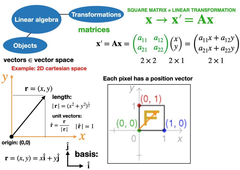
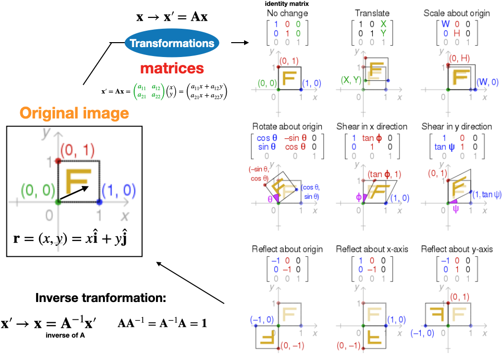
Transformation Matrices: Columns as Transformed Basis Vectors
Key insight the columns of \(A\) are exactly where the standard basis vectors \(\mathbf{e}_1, \mathbf{e}_2\) land after transformation.
\[A = \begin{pmatrix} a & b \\ c & d \end{pmatrix}, \quad \mathbf{e}_1 = \begin{pmatrix} 1 \\ 0 \end{pmatrix}, \quad \mathbf{e}_2 = \begin{pmatrix} 0 \\ 1 \end{pmatrix}\]
\[A\mathbf{e}_1 = \begin{pmatrix} a & b \\ c & d \end{pmatrix}\begin{pmatrix} 1 \\ 0 \end{pmatrix} = \begin{pmatrix} a \\ c \end{pmatrix} \leftarrow \text{column 1}\]
\[A\mathbf{e}_2 = \begin{pmatrix} a & b \\ c & d \end{pmatrix}\begin{pmatrix} 0 \\ 1 \end{pmatrix} = \begin{pmatrix} b \\ d \end{pmatrix} \leftarrow \text{column 2}\]
where \(\tilde{\mathbf{x}}\) denotes the transformed vector. Because \(A\mathbf{e}_1\) and \(A\mathbf{e}_2\) are just the images of the basis vectors (the columns of \(A\)), knowing where each basis vector goes (i.e., \(\mathbf{e}_1 \mapsto \tilde{\mathbf{e}}_1 = A\mathbf{e}_1\), \(\mathbf{e}_2 \mapsto \tilde{\mathbf{e}}_2 = A\mathbf{e}_2\)) tells you everything about how \(A\) transforms all vectors.
Matrix Inversion
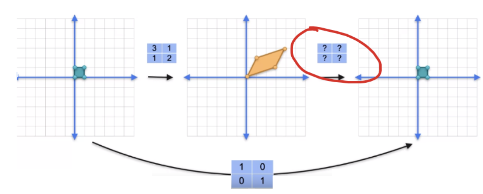
A square matrix \(A\) is invertible if there exists a matrix \(A^{-1}\) such that:
\[
A A^{-1}=A^{-1} A=I
\]
(where \(I\) is the identity matrix). A matrix has an inverse if and only if its determinant is non-zero ( \(\operatorname{det}(A) \neq 0\) ).
Common Methods for Computing Inverses
Analytic Methods (Exact / Formula-based): Best for small matrices ( \(2 \times 2\) or \(3 \times 3\) ) and theoretical proofs.
Adjugate Matrix Method (Cramer’s Rule): \(A^{-1}=\frac{1}{\operatorname{det}(A)} \operatorname{adj}(A)\). Computes the matrix of cofactors, transposes it, and divides by the determinant. Becomes computationally impossible for large matrices due to \(O(n!)\) or \(O\left(n^3\right)\) determinant calculations.
The Adjugate matrix is the transpose of the matrix of cofactors, where the cofactors are the determinants of the submatrices obtained by deleting the row and column of the element, multiplied by \((-1)^{i+j}\).
Numeric Methods (Algorithmic / Computer-based): Used by software for large, real-world matrices.
Gauss-Jordan Elimination: Convert the augmented matrix \([A \mid I]\) into \(\left[I \mid A^{-1}\right]\) using elementary row operations.
LU Decomposition: Decomposes \(A\) into lower \((L)\) and upper \((U)\) triangular matrices ( \(A= L U)\), then solves \(L U X=I\) using forward and backward substitution. This is the industry standard for computational efficiency ( \(O\left(n^3\right)\) complexity).
Numerical example: 2x2
np.linalg.inv(A) does numerical inversion using the LU decomposition method
Under the hood, np.linalg.inv(A) relies on highly optimized C and Fortran libraries called BLAS and LAPACK.
Specifically, it typically wraps LAPACK routines like _GESV (or _GETRF combined with _GETRI), which perform numerical matrix inversion using LU decomposition with
Simple \(2 \times 2\) Example To find the inverse of a \(2 \times 2\) matrix, swap the positions of \(a\) and \(d\), put negative signs in front of \(b\) and \(c\), and divide everything by the determinant \((a d-b c)\).
Step 3: Apply the Checkerboard of Signs (Matrix of Cofactors)
Apply a grid of alternating signs \(\begin{pmatrix} + & - & + \\ - & + & - \\ + & - & + \end{pmatrix}\) to the matrix of minors. This changes the sign of elements at \(M_{12}\), \(M_{21}\), \(M_{23}\), and \(M_{32}\):
Key intuition: invertibility is about whether \(A\) preserves the “richness” of space, singular matrices are the ones that irreversibly flatten it.
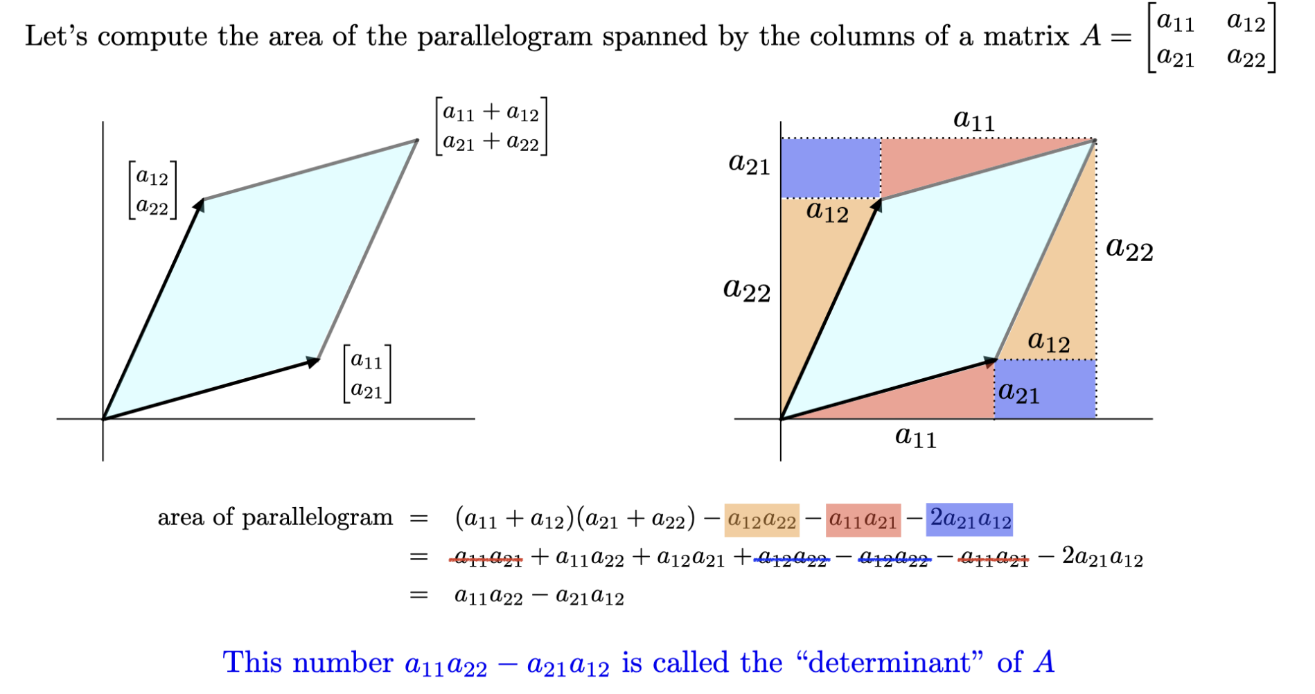
Transformed area
The two columns of \(A\) are the transformed basis vectors \(\tilde{\mathbf{e}}_1= (a_{11}, a_{21})^{\top}\) and \(\tilde{\mathbf{e}}_2=(a_{12}, a_{22})^{\top}\), which form a parallelogram.
The Determinant & Its Geometric Meaning
Algebraically a scalar \(\det(A)\) computed from an \(n \times n\) matrix that encodes whether \(A\) is invertible
Geometrically\(|\det(A)|\) is the factor by which \(A\) scales volume
\[\det\begin{pmatrix} a & b \\ c & d \end{pmatrix} = ad - bc\]
\(\det(A)\)
Meaning
\(= 0\)
\(A\) collapses space: not invertible
\(> 0\)
Volume scaled by \(\det(A)\), orientation preserved
\(< 0\)
Volume scaled by \(|\det(A)|\), orientation flipped
\(= 1\)
Volume unchanged (e.g., rotation)
2D example columns \(\mathbf{a}_1, \mathbf{a}_2\) form a parallelogram: \(|\det(A)|\) is its area
A square matrix \(A\) is invertible (i.e., has an inverse \(A^{-1}\)) if and only if the following equivalent statements hold
\(A\) is invertible (nonsingular)
\(\det(A) \neq 0\)
The equation \(A\mathbf{x} = \mathbf{0}\) has only the trivial solution (\(\mathbf{x} = \mathbf{0}\))
The columns of \(A\) are linearly independent
The columns of \(A\) span \(\mathbb{R}^n\)
The rank of \(A\) is \(n\)
\(A\) can be row reduced to the identity matrix
\(A\) has \(n\) pivot positions
The linear transformation \(\mathbf{x} \mapsto A\mathbf{x}\) is one-to-one and onto
The eigenvalue \(0\) is not an eigenvalue of \(A\)
All these conditions are equivalent for an \(n \times n\) matrix \(A\)! (If any one is true, all are true; if any one is false, all are false.)
Intuition behind the Invertible Matrix Theorem
All these conditions say the same thing \(A\) loses no information.
\(\det(A) \neq 0\): the matrix doesn’t collapse volume to zero; it stretches/rotates space without flattening it
\(A\mathbf{x} = \mathbf{0}\) has only \(\mathbf{x} = \mathbf{0}\): nothing gets “erased”; the only input that maps to zero is zero itself
Columns are linearly independent: no column is redundant; each one points in a genuinely new direction
Columns span \(\mathbb{R}^n\): the matrix can reach every point in space, so no output is “unreachable”
Rank \(= n\): all \(n\) dimensions are used; none are lost in the transformation
Row reduces to \(I\): \(A\) can be fully “undone” by elementary operations, confirming an inverse exists
\(n\) pivot positions: every row and column does independent work; no redundancy, no collapse
\(T\) is one-to-one and onto: distinct inputs give distinct outputs (one-to-one), and every output is reachable (onto); together, \(T\) is perfectly reversible
\(\lambda = 0\) is not an eigenvalue: if \(0\) were an eigenvalue, some nonzero vector would map to \(\mathbf{0}\), meaning \(A\) collapses space: exactly what invertibility forbids
Eigen vectors/values
Eigen vectors/values
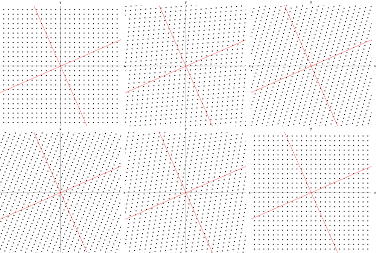
Visualization
A 2×2 real and symmetric matrix representing a stretching and shearing of the plane. The eigenvectors of the matrix (red lines) are the two special directions such that every point on them will just slide on them.
Solving an Eigenvalue Problem
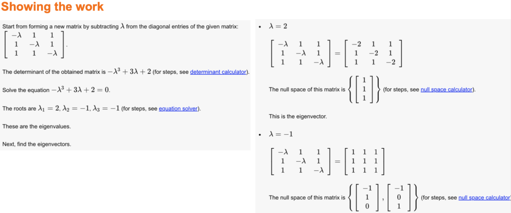
Set up\((A - \lambda I)\mathbf{x} = \mathbf{0}\): what scalars \(\lambda\) make \(A\) act like pure stretching?
Find eigenvalues via \(\det(A - \lambda I) = 0\): a nonzero solution exists only if \(A - \lambda I\) is singular
This is the Invertible Matrix Theorem flipped:
Finding eigenvalues is finding the \(\lambda\) values for which \(A - \lambda I\)fails the IMT: opening the door to nontrivial eigenvectors.
\[A \text{ invertible} \iff \det(A) \neq 0 \iff A\mathbf{x} = \mathbf{0} \text{ has only } \mathbf{x} = \mathbf{0}\]
\[\det(A - \lambda I) = 0 \iff (A - \lambda I) \text{ singular} \iff (A-\lambda I)\mathbf{x} = \mathbf{0} \text{ has a nonzero solution}\]
Find eigenvectors by substituting each \(\lambda\) back: the null space of \(A - \lambda I\) reveals which directions are purely stretched
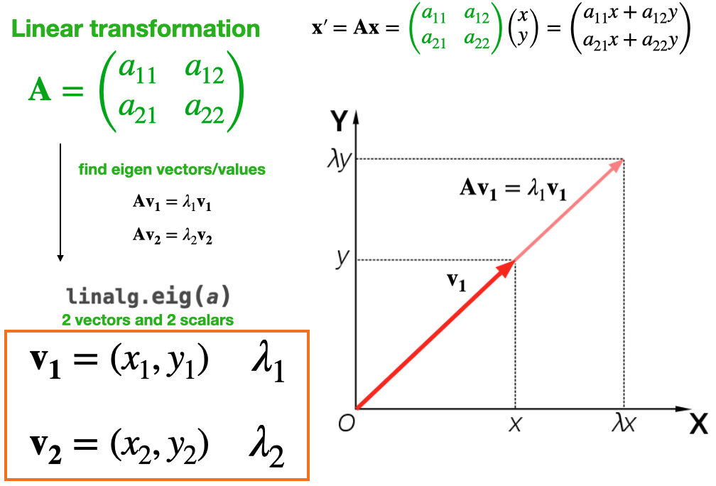
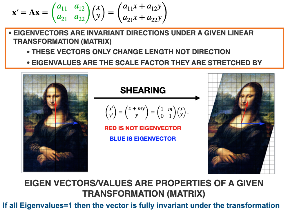
Interpret each \((\lambda, \mathbf{x})\) pair: \(\mathbf{x}\) is a direction \(A\) leaves invariant, scaled by \(\lambda\)
Left and Right Eigenvalue Problems
A right eigenvector is a direction that \(A\) merely stretches when acting on column vectors from the left \((A \mathbf{x}=\lambda \mathbf{x})\), while a left eigenvector is a row vector that gets stretched when it acts on \(A\) from the left ( \(\mathbf{y}^{\top} A=\lambda \mathbf{y}^{\top}\) ), same eigenvalues, just the matrix acting from opposite sides.
Running example \(A = \begin{pmatrix} 2 & 1 \\ 0 & 3 \end{pmatrix}\), with eigenvalues \(\lambda = 2, 3\)
Row vector \(\mathbf{y}^\top\), multiplied on the left of \(A\)
Equivalent to a right eigenvector of \(A^\top\)
Key facts
Same eigenvalues \(\lambda\) in both problems
If \(A\) is symmetric, left and right eigenvectors coincide
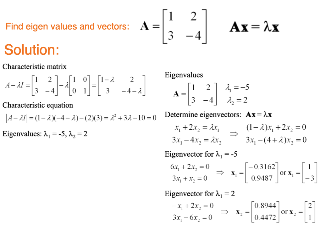
Analytic example: Eigenvalue Problem
The characteristic polynomial \(\det(A - \lambda I)\) is always degree \(n\) for an \(n \times n\) matrix, giving exactly \(n\) eigenvalues (counting multiplicity, over \(\mathbb{C}\)). One stretching direction per dimension of the space.
Notice that there are \(n\) eigenvalues and \(n\) eigenvectors, one per dimension of the space.
Looking ahead: Adjacency matrix
IMPORTANT: Whenever you encounter a well-defined, mathematically meaningful square matrix—especially one with a clear real-world interpretation—it makes sense to analyze its eigenvectors. Examples include the adjacency matrix, covariance matrix, and others.
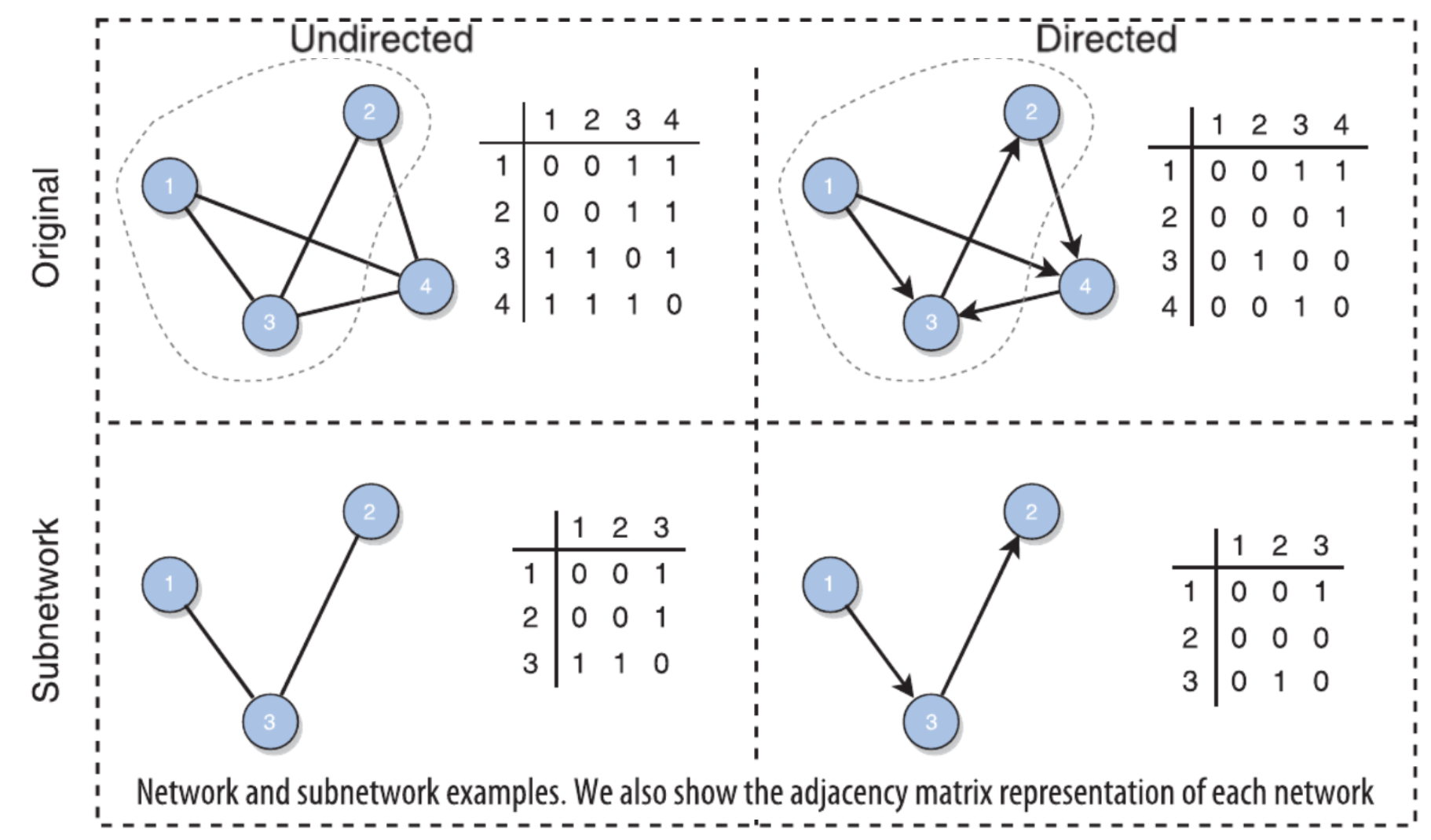
Element \(a_{i j}\) of the adjacency matrix represents the link between nodes \(i\) and \(j . a_{i j}=1\) if \(i\) and \(j\) are adjacent, \(a_{i j}=0\) otherwise.
When you encounter a square matrix, particularly if it has a well defined real-world interpretation, it is logical to analyze the Eigen-vectors.
Famous square matrices:
The Adjacency Matrix (Network Science & ML): Defines connections between nodes in a graph; its principal eigenvector yields eigencentrality scores, which rank nodes based on their overall influence and connectivity within the network.
The Covariance Matrix (Machine Learning): Yields the principal components (eigenvectors), which identify the directions of maximum variance in a dataset for dimensionality reduction (PCA).
The Inertia Tensor (Physics): Identifies the principal axes of inertia (eigenvectors), showing the specific axes about which an object can rotate cleanly without wobbling.
The Graph Laplacian (Machine Learning & Network Science): Reveals structural network partitions; the eigenvector corresponding to the second-smallest eigenvalue provides the mathematically optimal way to split a graph into communities (Spectral Clustering).
The Hessian Matrix (Machine Learning): Determines the local curvature of a loss function landscape, where the signs and magnitudes of the eigenvalues identify whether a point is a minimum, maximum, or saddle point.
The Hamiltonian Matrix (Physics): Solves the Schrödinger equation, where the eigenvalues provide the exact allowed energy levels of a quantum system and the eigenvectors represent its stable quantum states.
The Density Matrix (Quantum Mechanics & Quantum ML): Allows for the extraction of pure states from a statistical mixture and is used to compute Von Neumann entropy to measure quantum entanglement.
The Stress Tensor (Physics): Uncovers the principal stress directions (eigenvectors), indicating the precise planes of maximum tension or compression where a material is most likely to fracture.
Eigen-centrality
The Spectral Theorem: Why Symmetry Is a Gift in Network Analysis
The spectral theorem says any real symmetric matrix has all real eigenvalues and a full set of orthogonal eigenvectors, so it can be written as \(A = Q\Lambda Q^{T}\): a clean rotation into a coordinate system where the matrix is just a diagonal stretch.
Why networks care: undirected graphs have symmetric adjacency and Laplacian matrices, so the theorem applies and the eigenvectors become a natural basis for any signal living on the nodes.
It is the bedrock under a huge amount of method. Eigenvector centrality is well-posed (a unique, real, positive leading eigenvector), spectral clustering and graph partitioning split the graph along the low-eigenvalue eigenvectors, and diffusion, heat kernels, and random walks all decompose cleanly into independent eigen-modes.
The intuition: orthogonal eigenvectors are non-interfering directions. A process on the graph can be broken into independent modes that each just decay or grow at their own rate, which is what makes the analysis tractable.
The catch, and the thread through this unit: direction breaks symmetry. An asymmetric adjacency matrix can have complex eigenvalues, may not diagonalize, and splits left from right eigenvectors. Losing the spectral theorem is precisely why directed eigenvector centrality misbehaves and why fixes like Katz and PageRank exist.
Overview
Eigen-centrality is a prestige score which measures the node’s influence
It is a nodal attribute, as is the case with all other centrality measures.
Connections to high-scoring nodes contribute more to the score of the node in question than equal connections to low-scoring nodes
A high Eigen-centrality means the node is connected to many nodes with high scores.
Google’s PageRank and the Katz centrality are variants of the eigenvector centrality.
Big picture
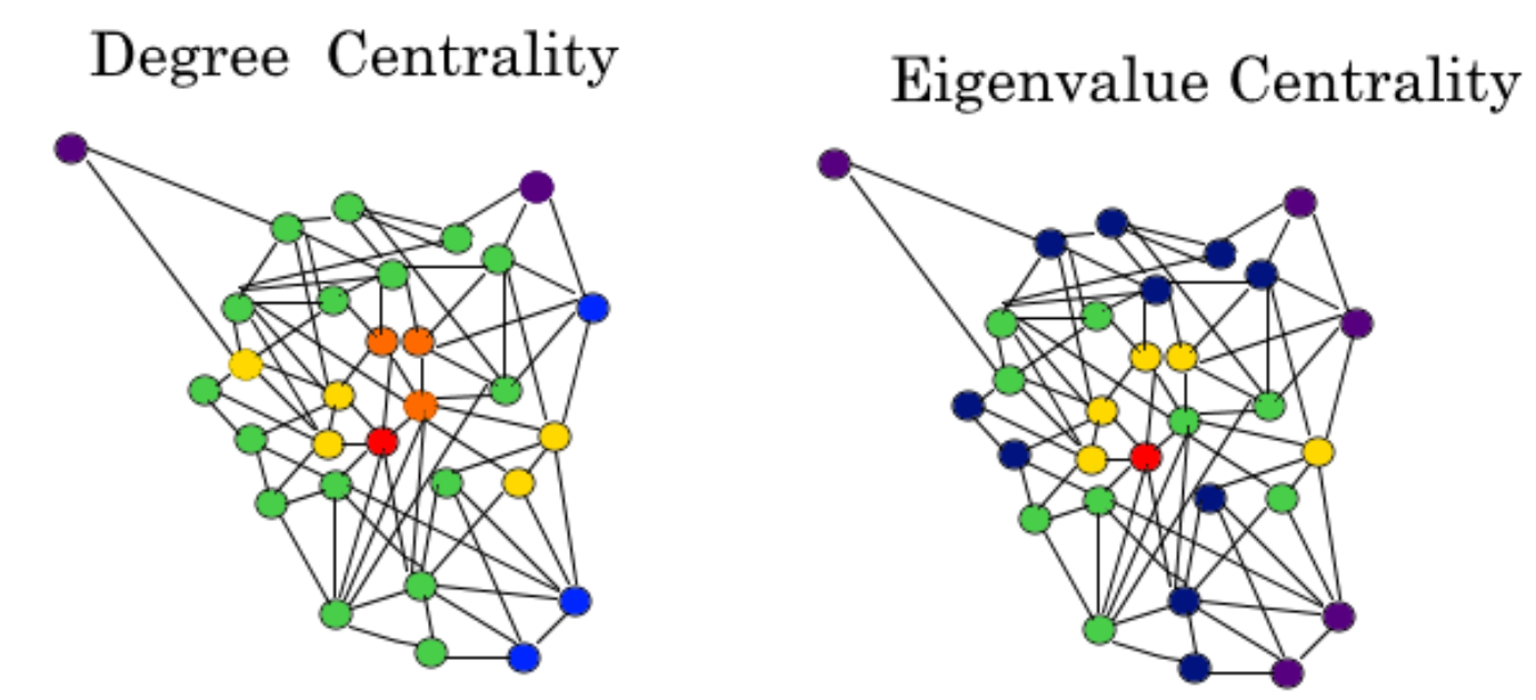
Degree centrality asks how many connections does a node have?
Eigenvector centrality asks a deeper question how important are the nodes you are connected to?
Core intuition a node is important if it is connected to other important nodes
The definition is recursive, your score depends on your neighbors’ scores, which depend on their neighbors’ scores, and so on
Classic analogy being friends with 10 well-connected people may matter more than being friends with 50 isolated people
Why It Matters
Captures influence, not just popularity
Social networks a person followed by celebrities vs. a person followed by bots
Citation networks being cited by landmark papers vs. obscure ones
Foundation for famous algorithms
PageRank (Google) and Katz centrality are direct descendants
Used in epidemiology (super-spreaders), economics (systemic risk), neuroscience (hub regions)
Dimensionality of the Eigencentrality Vector
For a network with \(n\) nodes, the adjacency matrix \(A\) is \(n \times n\), and the eigenvector equation is:
\(\mathbf{x}\) has one entry per node, the eigencentrality of node \(i\) is simply the scalar \(x_i\)
The full vector \(\mathbf{x} = (x_1, x_2, \ldots, x_n)^\top\) is the centrality profile of the entire network
The degree of the characteristic polynomial is \(n\), so there are \(n\) eigenvector solutions, one per dimension of the network
Intuition: the eigenvector lives in “node space”, each axis corresponds to a node, and the eigenvector assigns a score along each axis simultaneously, subject to the self-consistency condition across the whole network.
Setting Intuition for Eigenvector Centrality
Core idea: a node is important if it is connected to other important nodes, importance is self-referential.
Setup: let \(x_i\) be the centrality of node \(i\). We want each node’s score to be proportional to the sum of its neighbors’ scores:
This is a self-consistency condition: we seek a centrality assignment where every node’s score is simultaneously explained by its neighbors’ scores, which are explained by their neighbors, and so on.
We don’t assume neighbors have similar scores
We look for a global fixed point: an assignment that wouldn’t change if you recomputed every node from its neighbors at once
The eigenvalue \(\lambda\) is simply the scaling factor that makes this balance globally
This is exactly what the eigenvector equation captures: the one centrality vector stable under the entire network’s structure.
Definition
Let \(A\) be the adjacency matrix of an undirected graph, where \(A_{ij} = 1\) if nodes \(i\) and \(j\) are connected.
The centrality \(x_i\) of node \(i\) is proportional to the sum of its neighbors' centralities
By the Perron–Frobenius theorem, choosing \(\lambda = \lambda_{\max}\) (the largest eigenvalue) guarantees an eigenvector with all non-negative entries, the only choice that makes sense as a centrality score
Scores are typically normalized so that \(\lVert \mathbf{x} \rVert_2 = 1\)
Eigencentrality ranks nodes recursively: “You are important if other important nodes link to you.” This maps to the eigenvector equation \(Av = \lambda v\), where \(A\) is the adjacency matrix.
The Perron–Frobenius Theorem is the mathematical guarantee that this recursive definition yields a valid, stable ranking.
The 3 Core Guarantees
For any strongly connected network (where every node can reach every other node), the theorem guarantees that the matrix \(A\):
Has a Unique Maximum: Possesses a single, unique largest real eigenvalue (\(\lambda_{\max}\)).
Yields Positive Scores: The corresponding principal eigenvector \(v\) has strictly positive components (\(v_i > 0\)). Every node receives a meaningful, non-zero score.
Is Unambiguous: No other positive eigenvectors exist, ensuring a definitive ranking.
The Directed Graph Problem (Sinks & Dead Ends)
Undirected Graphs: If connected, they naturally meet the theorem’s criteria.
Directed Graphs: Often break the theorem because they contain sinks (nodes with incoming edges but no outgoing edges).
Without outgoing edges to recirculate influence, the matrix loses its mathematical “irreducibility.” Consequently, the Perron–Frobenius guarantees collapse, and the centrality scores of entire clusters can drain away, dropping to zero. This fatal flaw is why PageRank introduces a “damping factor” (random teleportation)—it artificially restores strong connectivity so the Perron–Frobenius theorem can function properly.
NetworkX
The following command computes the eigenvector centrality for the graph \(\mathrm{G}\).
Eigenvector centrality computes the centrality for a node based on the centrality of its neighbors.
The eigenvector centrality for node \(i\) is the \(i\)-th element of the vector \(x\) defined by the equation \[
A x=\lambda x
\]
where \(A\) is the adjacency matrix of the graph \(\mathrm{G}\) with eigenvalue \(\lambda\).
By virtue of the Perron-Frobenius theorem, there is a unique solution \(x\), all of whose entries are positive, if \(\lambda\) is the largest eigenvalue of the adjacency matrix \(A\).
Example
Code
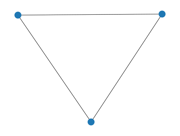
import networkx as nximport numpy as np# CREATE-1G=nx.complete_graph(3)# CREATE-2# G = nx.DiGraph()# G = nx.Graph()# G.add_nodes_from([0,1,2,3,4])# G.add_edges_from([(0, 1), (0, 2), (0,3), (0,4),(1,0),(2,3)])# DRAWnx.draw(G)# ADJACENCY MATRIXA=nx.adjacency_matrix(G).todense()print("Adjacency matrix\n",A)# METHOD-1: NETWORKX EIGENVECTOR_CENTRALITYprint("\nEIGENVECTOR_CENTRALITY:\n",nx.eigenvector_centrality(G))# METHOD-2: COMPUTE FROM "SCRATCH"print("EIGENVALUES:",np.linalg.eig(A)[0])eVect=np.array(np.linalg.eig(A)[1])print("\nEIGENVECTORS:\n",np.round(eVect,4))print("LENGTH OF EIGEN VECTORS:",np.sqrt(np.sum((eVect)**2,axis=0))**0.5)
For directed graphs this is “left” eigenvector centrality which corresponds to the in-edges in the graph. For out-edges eigenvector centrality first reverse the graph with G.reverse().
Code
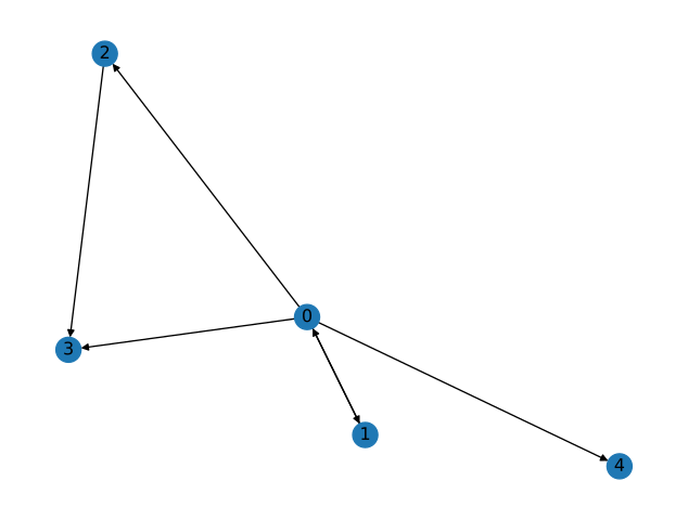
# Generate graphimport networkx as nxG = nx.DiGraph()G.add_nodes_from([0,1,2,3,4])G.add_edges_from([(0, 1), (0, 2), (0,3), (0,4),(1,0),(2,3)])nx.draw(G,with_labels=True)# ADJACENCY MATRIXA=nx.adjacency_matrix(G).todense().T #TRANSPOSE MAKES IT IN-DEGREE ORIENTS ROWS=INprint("Adjacency matrix\n",A)# METHOD-1: NETWORKX EIGENVECTOR_CENTRALITYprint("\nEIGENVECTOR_CENTRALITY:\n",nx.eigenvector_centrality(G))# METHOD-2: COMPUTE FROM "SCRATCH"print("EIGENVALUES:",np.linalg.eig(A)[0])eVect=np.array(np.linalg.eig(A)[1])print("\nEIGENVECTORS:\n",np.round(eVect,4))print("LENGTH OF EIGEN VECTORS:",np.sqrt(np.sum((eVect)**2,axis=0))**0.5)
Eigencentrality works best for undirected graphs because they always yield a symmetric matrix with a clear, guaranteed principal eigenvector, whereas directed graphs can produce asymmetric matrices where centrality scores fail to properly propagate backward from “dead ends” or sinks.
Localization in networks with large hubs, nearly all the centrality mass can concentrate on the hub and its neighbors, leaving the rest of the network with scores near zero
Directed graphs nodes with no incoming edges get a score of exactly 0, and they pass that zero along, so entire regions of a DAG can score 0 (motivates Katz centrality, which adds a baseline score \(\beta\) to every node)
Disconnected graphs scores are only meaningful within a single connected component; the leading eigenvector concentrates on one component
Convergence power iteration can converge slowly (or fail) on some graphs, e.g., bipartite structures where \(|\lambda_1| = |\lambda_2|\)
No cross-network comparison scores are normalized per-graph, so values are not comparable across different networks
Summary
Eigenvector centrality scores nodes by the importance of their neighbors, not just their count
Mathematically the leading eigenvector of the adjacency matrix, \(A\mathbf{x} = \lambda_{\max}\mathbf{x}\)
Easy to compute (nx.eigenvector_centrality), and the basis for Katz centrality and PageRank
Best suited to connected, undirected networks; use Katz/PageRank for directed graphs