import plotly.io as pio
pio.renderers.default = "plotly_mimetype+notebook_connected"Plotly
—; title: ‘Plotly: Client-side interactive visualization’
Overview and introduction
Recall: Client vs server
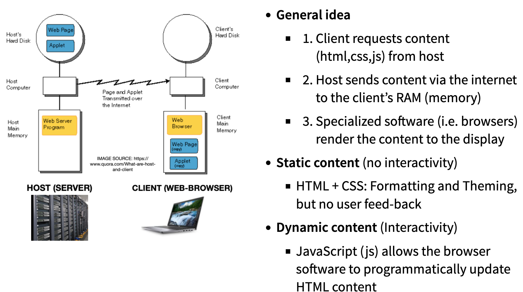
Recall: General idea behind interactive graphics

What is Plotly?
- Plotly is a technical computing company headquartered in Montreal, Canada

- The company develops tools for data visualization, analytics, and statistical tools, as well as graphing libraries for Python, R, MATLAB, Perl, Julia, Arduino, and REST.
The Plotly tool suite
- Dash: An open-source framework (primarily Python, with R and Julia bindings) for building interactive analytic web applications.
- Dash Enterprise: Plotly’s commercial platform for building, testing, deploying, managing, and scaling Dash applications in enterprise environments.
- Chart Studio Cloud: A hosted, point-and-click graph authoring tool for creating interactive Plotly charts online.
- Chart Studio Enterprise: A self-hosted, paid version of Chart Studio for teams, offering advanced authentication, permissions, and sharing controls.
- Data visualization libraries
- Plotly.js is the core open-source JavaScript library for creating interactive graphs. Official wrappers are available for Python, R, Julia, and MATLAB.
- Figure converters Tools that convert matplotlib and ggplot2 figures into interactive Plotly figures.
Where do we stand?
- Today we focus on the client side libraries, which wrap
plotly.jsfor R and Python.
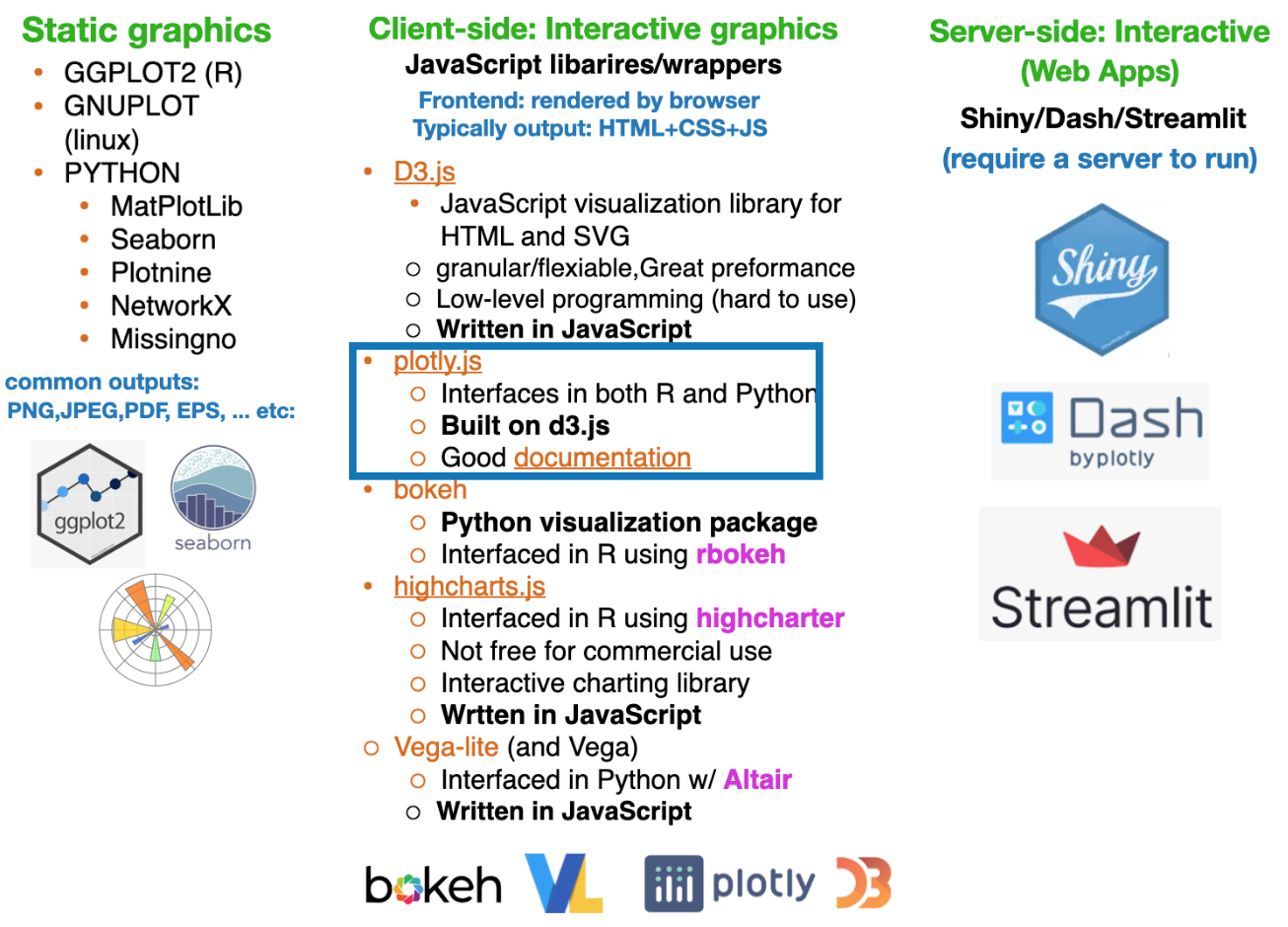
Plotly.js and D3.js: How They’re Connected
- Plotly.js is built on top of D3.js, using it for DOM manipulation, data binding, and SVG rendering
- D3.js is an internal dependency, not part of Plotly.js’s public API
- Plotly.js adds a high-level, declarative charting layer on top of D3
- WebGL is also used for high-performance rendering of large datasets
- WebGL is a browser-based graphics API that enables high-performance 2D and 3D rendering by executing GPU-accelerated graphics directly within web applications.
Bottom line: Plotly.js leverages D3.js internally, but abstracts away its low-level complexity for end users.
Plotly.js: Interactive controls
Plotly plots have interactive controls, shown in the top-right, to do the following:

- Pan: Move around in the plot.
- Box Select: Select a rectangular region of the plot to be highlighted.
- Lasso Select: Draw a region of the plot to be highlighted.
- Autoscale: Zoom to a “best” scale.
- Reset axes: Return the plot to its original state.
- Toggle Spike Lines: Show or hide lines to the axes whenever you hover over data.
- Show closest data on hover: Show details for the nearest data point to the cursor.
- Compare data on hover: Show the nearest data point to the x-coordinate of the cursor.
Source: click here
Why Interactive Visualization Matters
Interactivithy introduces a new dimension of story-telling (author driven vs user driven)
- Reveals structure in data that static charts can hide (outliers, clusters, trends)
- Supports real-time exploration, not just presentation, enabling users to ask follow-up questions in real time
- Reduces cognitive load through tooltips, filtering, and selective emphasis
- Scales to higher-dimensional data using color, size, facets, and interaction
- Bridges analysis and communication, allowing the same figure to serve analysts and stakeholders
Aside: Free & Popular Data-Driven Storytelling Sites
These can be used for inspiration for your projects
The Pudding – A standalone data storytelling site with deeply interactive, explanatory articles on culture, sports, and social trends, built around data narratives and visual exploration. ([The Pudding][1])
FlowingData – A long-running visualization site by Nathan Yau combining analysis, charts, and narrative to help explain insights from data in engaging ways. ([Blogs Database][2])
DataJournalism.com – A central hub for data journalism practitioners and learners, featuring free resources, case studies, and links to standout projects (not a single “story,” but a repository of many). ([DataJournalism.com][3])
Interactive data storytelling projects via Flourish – While not a single traditional “website,” Flourish’s gallery showcases free, embeddable interactive visualizations (e.g., bar chart races, scrollytelling) that exemplify modern data storytelling techniques. ([Flourish][4])
Awesome Interactive Journalism (GitHub curation) – A community-maintained list linking to a broad set of free interactive journalism and data storytelling projects from around the web. ([GitHub][5])
Core Plotly Constructs
- Figure – The top-level object; contains everything.
- Trace – A single chart layer (scatter, bar, line, heatmap, etc.).
- Data Arrays – The values bound to a trace (
x,y,z,values). - Layout – Global configuration (axes, titles, legends, margins).
- Axes – Scale, range, ticks, labels, and coordinate system.
- Visual Encodings – Marker, line, color, size, opacity.
- Interactivity – Hover, zoom, pan, select, legend toggling (built-in).
- Subplots – Multiple plots in one figure.
- Templates – Reusable styling defaults.
- Renderer – SVG (small/precise) vs WebGL (large/high-performance).
Rule of thumb: You build figures by adding traces to a figure and controlling behavior via layout.
Example-1: Plotly.js
- We already interacted a bit with
Plotly.jsin pureJavaScriptform in Lab-3.1 - Many of the elements in pure
JavaScriptversion of Plotly, such as traces, layout, and data, are also mirrored in the Python and R wrappers that we will see later.

Plotly.js: Fundamental components
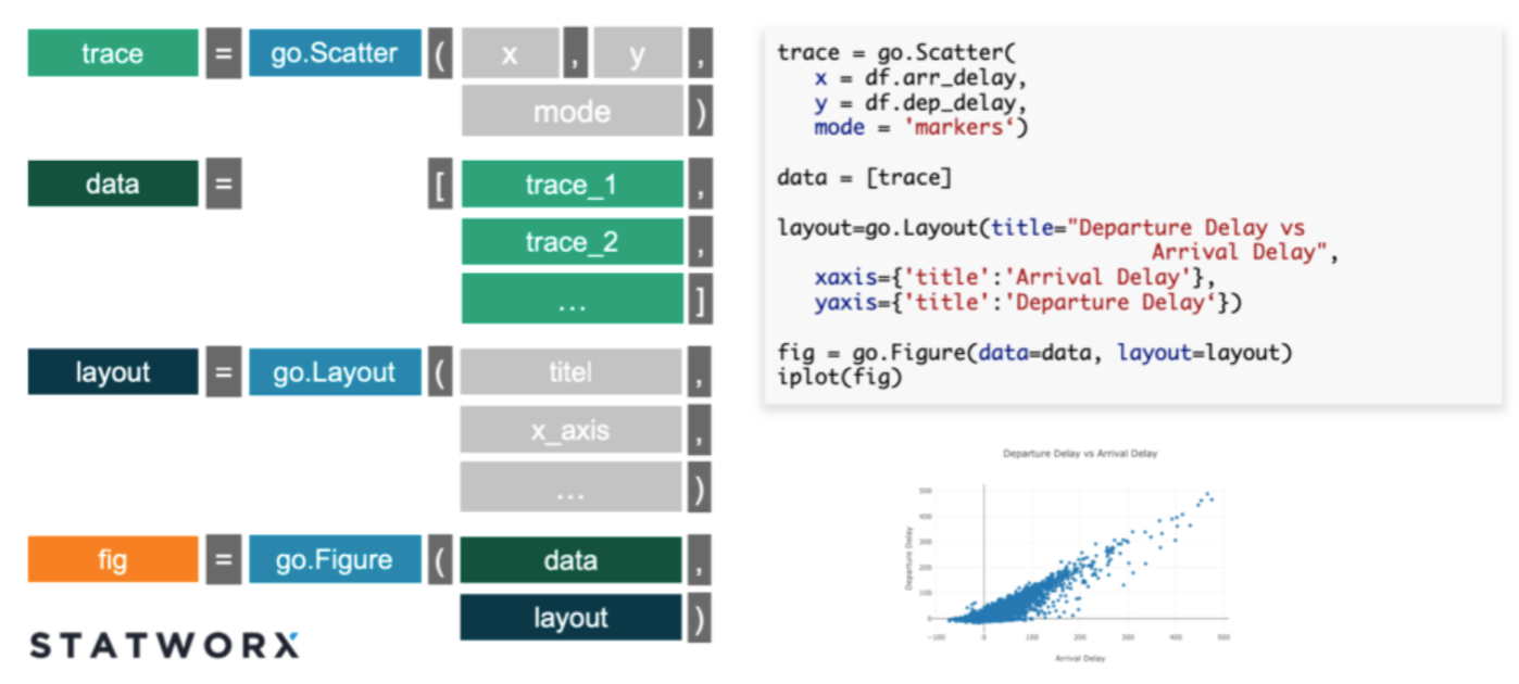
- Trace: Describes a collection of data and the specifications about how you want the data displayed on the plotting surface, which is described by the
trace type(scatter, box, , etc). - Data: Collection (list) of traces
- Layout: Controls various structural and stylistic components of the figure (e.g. title, font, size, etc)
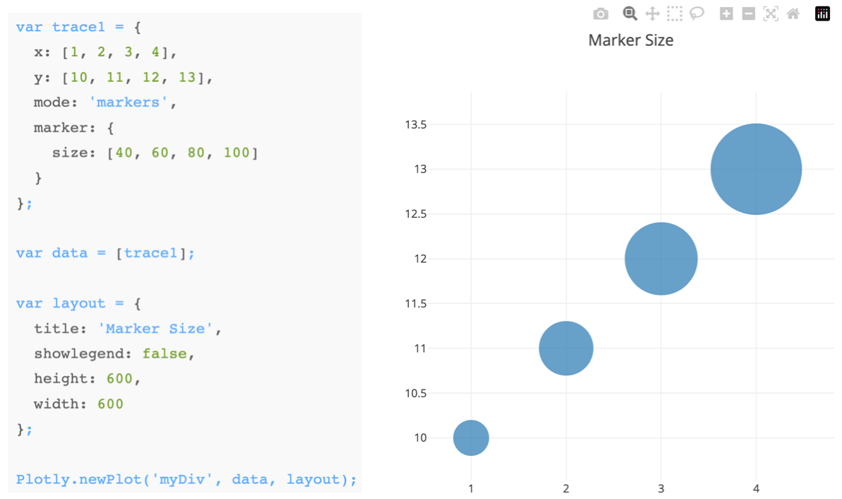
The Python (or R) wrappers create JSON files that map from python commands to the format needed by plotly.js with these fundamental components
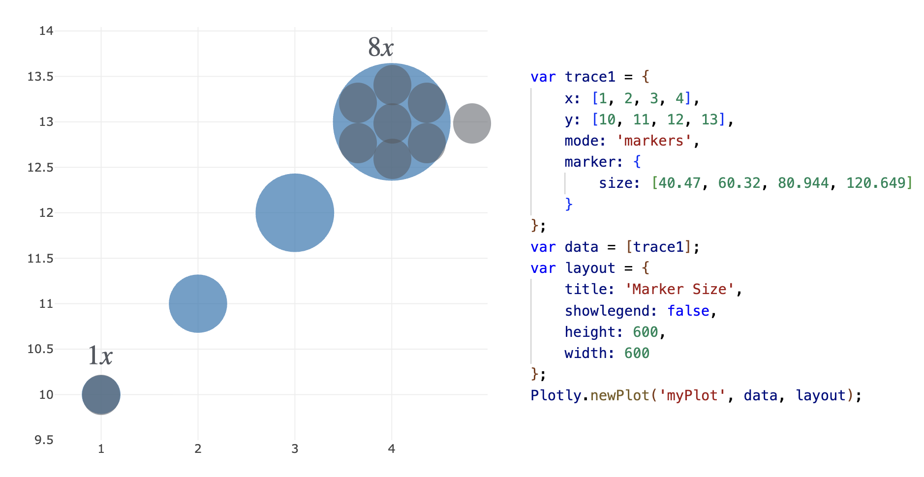
As always, keep your geometry in mind
Original data encoded as marker size:
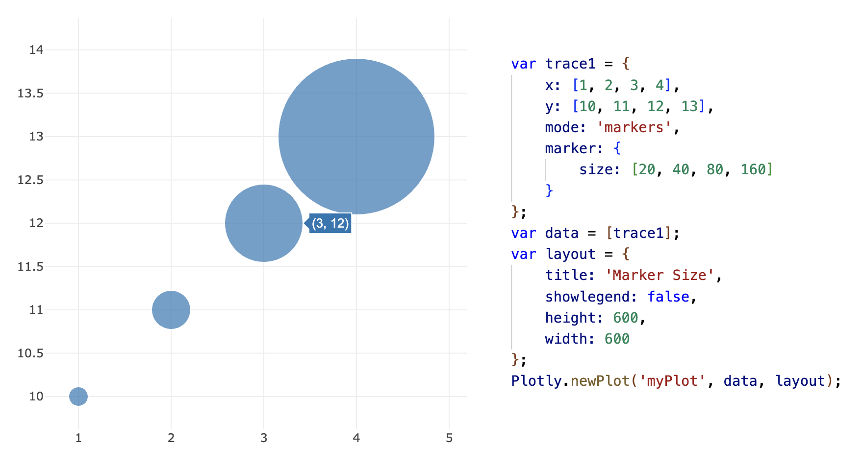
Square root transformation:
Plotly in Python
Introduction to plotly.py
How does Plotly.py work?
- Let’s start on the python side for the sake of explanation
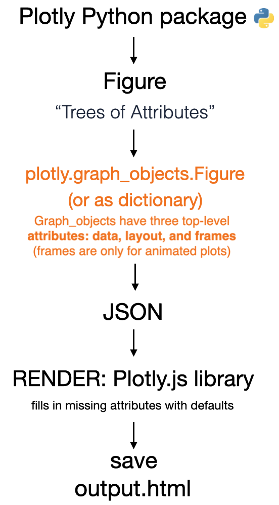
- Similar to MPL, The fundamental Plotly data-structure is the
Plotly figure(i.e. charts, plots, maps and diagrams)- Figures are represented as dictionaries or as instances of the plotly.graph_objects.Figure class
- Python exports the Figure object to a
JSON fileto be rendered byplotly.js.
Source: click here
Constructing a graph
- When using Plotly in python there are generally two ways to create graphs.

- Easy method: The high-level
plotly.expressmodule which is a set of Python functions to return completed plotly.graph_objects.Figure objects. - Advanced method: Plotly
graph_objectsmodule which has more control, customization, and understanding of whats happening “under the hood”
Plotly express vs Graph objects
Plotly Express is a better starting point for plot creation, since it is powerful and easy
Plotly Express functions use graph objects internally and return a plotly.graph_object
- Therefore, you can also switch at any point to working as a graph_object
It is good to use the graph_objects module in the following cases:
Non-standard visualizations: It is difficult to create non-standard graphs with Plotly Express, therefore graph_objects must be used
When you have a lot of customizations: If you want to make a lot of changes to most aspects of your charts, you might end up writing the same amount of code and putting in the same amount of effort, so you might consider doing it directly using the graph_objects module.
Sub-plots: Sometimes you want to have multiple charts side by side, or in a grid. If these are different charts and not facets, then it’s better to do with graph_objects.
Aside: Embedding HTML into documents
- When using Quarto or Jupyter notebook, often we want to embed individual HTML files (e.g. Plotly output files) into our documents.
- There are multiple ways to do this;
- If using
.qmdor.rmdusually the figures will render correctly “inline” without saving the file or adding more code - If using
.ipynbsometimes the rendering can be buggy, especially in VS-code. If it doesn’t render correctly then you can do the following.- save the image as html to a file
- re-embed it into the document as an iframe
- You can embed in markdown using inline-html (recommended)
<iframe src="file_name.html" height="1000" width="1000"></iframe>
- Alternatively, you can also embed it using python commands (see next slide)
Aside: Embedding HTML into documents
Additionally, you can embed in python using the following commands, however the markdown+HTML option is recommended.
# CREATE FIGURE OBJECT
import plotly.express as px
fig = px.line(x=["a","b","c"], y=[1,3,2], title="sample figure")

# SAVE TO FILES
file_name="./img/plotly-0.html"
fig.write_html(file_name)

# RE-LOAD AS AN IFRAME
from IPython.display import IFrame
IFrame(src=file_name, width=375, height=700)
Aside: Plotly in VS-code inside .ipynb
- If you are using Plotly within the VS Code Notebook Editor you will need to add a line of code to ensure that your plots can be seen both within VS Code and when rendered to HTML by Quarto.
- Note that this workaround is only required for the VS Code Notebook Editor (it is not required if you are using Jupyter Lab or if you are editing a plain-text .qmd file).
- You can do this by configuring the Plotly default renderer as follows:
Source: click here
Example: MPL to Plotly conversion
- We can recycle our old plots, but add interactivity, using
plotly.toolsconverters.
- The conversion is done with
fig = tls.mpl_to_plotly(mpl_fig)fromimport plotly.tools as tls
# import warnings
# warnings.filterwarnings("ignore")

# IMPORT MODULES
import numpy as np
import matplotlib.pyplot as plt
import plotly.tools as tls

# CREATE DATA ARRAYS
x = np.linspace(-2.0 * np.pi, 2.0 * np.pi, 51)
y = np.sin(x)

# MAKE A MPL FIGURE
mpl_fig = plt.figure()
plt.plot(x, y, "ko--")
plt.xlabel("x")
plt.ylabel("sin(x)")
# plt.show()

# CONVERT USING PLOTLY
fig = tls.mpl_to_plotly(mpl_fig)

# UPDATE THEME
fig.update_layout(template="plotly_white")
fig.update_layout(width=800, height=400)

# SHOW
fig.show()

# # # SAVE AND RENDER
# file_name="./img/mpl-to-plotly.html"
# fig.write_html(file_name)
# from IPython.display import IFrame
# IFrame(src=file_name, width=900, height=500)
Plotly.py
Getting started with Plotly express
Note: Repeated package imports are intentional to make the code cells self contained
Plotly Express: function arguments
- The input arguments for a Plotly express function are similar to other libraries.
- The typical data input is a Pandas data frame, list, or numpy array
- The x argument is a string naming the column to be used on the x-axis.
- The y argument can either be a string or a list of strings naming column(s) to be used on the y-axis.
- Basic customization is straight-forward

- IMPORTANT: To make stylistic changes, e.g. figure-size, we can use
fig.update_layout()
Source: click here
Plotly Express: Available functions
- Basics:
scatter,line,area,bar,funnel,timeline - Part-of-Whole:
pie,sunburst,treemap,icicle,funnel_area - 1D Distributions:
histogram,box,violin,strip,ecdf - 2D Distributions:
density_heatmap,density_contour,imshow - 3-Dimensional:
scatter_3d,line_3d - Multidimensional:
scatter_matrix,parallel_coordinates,parallel_categories - Tile Maps:
scatter_mapbox,line_mapbox,choropleth_mapbox,density_mapbox - Outline Maps:
scatter_geo,line_geo,choropleth - Polar Charts:
scatter_polar,line_polar,bar_polar - Ternary Charts:
scatter_ternary,line_ternary
Source: click here
The Gap-minder data-set
- In the following examples, we will be using the well known
gapminderdata-set - The Gapminder is a comprehensive data set containing information on global demographics, economics, health, and social indicators over time.
- Let’s take a quick look
import plotly.express as px

df = px.data.gapminder()
df = df.drop(["iso_num"], axis=1)  # DROP COLUMN
print("Shape =", df.shape, "\n")
print(df.head())
Shape = (1704, 7)
country continent year lifeExp pop gdpPercap iso_alpha
0 Afghanistan Asia 1952 28.801 8425333 779.445314 AFG
1 Afghanistan Asia 1957 30.332 9240934 820.853030 AFG
2 Afghanistan Asia 1962 31.997 10267083 853.100710 AFG
3 Afghanistan Asia 1967 34.020 11537966 836.197138 AFG
4 Afghanistan Asia 1972 36.088 13079460 739.981106 AFGThe Tips data-set
- In the following examples, we will also be using the well known
Tipsdata-set - This dataset contains information on the tips collected by a restaurant waiter during different shifts. It includes information about the total bill, the tip amount, the gender of the person paying, whether they smoked or not, the day of the week, the time of day, the size of the group, and the type of meal (lunch or dinner).
- Let’s take a quick look
import plotly.express as px
import seaborn as sns

tips = px.data.tips()
print(tips)
total_bill tip sex smoker day time size
0 16.99 1.01 Female No Sun Dinner 2
1 10.34 1.66 Male No Sun Dinner 3
2 21.01 3.50 Male No Sun Dinner 3
3 23.68 3.31 Male No Sun Dinner 2
4 24.59 3.61 Female No Sun Dinner 4
.. ... ... ... ... ... ... ...
239 29.03 5.92 Male No Sat Dinner 3
240 27.18 2.00 Female Yes Sat Dinner 2
241 22.67 2.00 Male Yes Sat Dinner 2
242 17.82 1.75 Male No Sat Dinner 2
243 18.78 3.00 Female No Thur Dinner 2
[244 rows x 7 columns]Plotly-express hello world: scatter-plot
- Here is a very basic example using the defaults
import plotly.express as px
import seaborn as sns

# GET DATA
df = sns.load_dataset("penguins")
# print(df.keys())

# GENERATE PLOTLY FIGURE
fig = px.scatter(
    data_frame=df,
    x="bill_length_mm",
    y="body_mass_g",
)

fig.show()
Basic customization
- Now lets add some basic customization.
import plotly.express as px
import seaborn as sns

# GET DATA
df = sns.load_dataset("penguins")
# print(df.keys())
df = df.dropna()  # drop rows with nan

# GENERATE PLOTLY FIGURE
fig = px.scatter(
    data_frame=df,
    x="bill_length_mm",
    y="body_mass_g",
    # color="body_mass_g",
    color="species",
    template="plotly_white",  # THEME
    labels={"body_mass_g": "Body mass (grams)", "bill_length_mm": "Bill length (mm)"},
    title="Visualization of penguins species phenotypical clustering",
)
# MAKE POINTS LARGER AND CHANGE FONT
fig.update_traces(marker_size=14)
fig.update_layout(font={"size": 18})

# SHOW
fig.show()
Modified version
- The following produces the same plot, but from a list instead of a data frame
- Notice the color-palette automatically changes for qualitative vs quantitative variables
import plotly.express as px
import seaborn as sns

# GET DATA
df = sns.load_dataset("penguins")
# print(df.keys())
df = df.dropna()  # drop rows with nan
# print(list(df["bill_length_mm"]))

# GENERATE PLOTLY FIGURE
fig = px.scatter(
    x=list(df["bill_length_mm"]),
    y=list(df["body_mass_g"]),
    color=list(df["body_mass_g"]),
    template="plotly_white",  # THEME
    labels={"x": "Body mass (grams)", "y": "Bill length (mm)"},
    title="Visualization of penguins species phenotypical clustering",
)
# MAKE POINTS LARGER AND CHANGE FONT
fig.update_traces(marker_size=14)
fig.update_layout(font={"size": 18}, height=450)

# SHOW
fig.show()
Example: Plotting a dictionary object
- We can also plot from a dictionary data structure
- To plot from a dictionary, the x and y are typically stored as list (or numpy arrays).
# GENERATE PLOTLY FIGURE OBJECT
import plotly.express as px
import numpy as np

dict = {"dates": ["2020-01-01", "2020-01-02", "2020-01-03", "2020-01-04"], "y_vals": np.array([100, 200,300,400])}
fig = px.scatter(dict, x="dates", y="y_vals")

fig.update_layout(height=400, width=600)

fig.show()
Pair-plot: Default
As usual with most packages, the default styling is quite bad
import plotly.express as px
import seaborn as sns

penguin = sns.load_dataset("penguins")

fig = px.scatter_matrix(penguin, width=500, height=500)
fig.show()
Pair-plot: Customized
Even just a few minor tweaks brings the graph much closer to publication quality
# Import necessary libraries
import plotly.express as px
import seaborn as sns

# Load the penguins dataset from seaborn
df = sns.load_dataset("penguins")

# Create a scatter matrix (pair plot) using selected dimensions (columns)
fig = px.scatter_matrix(
    df,
    dimensions=[
        "bill_length_mm",    # Penguin bill length in mm
        "bill_depth_mm",     # Penguin bill depth in mm
        "flipper_length_mm", # Penguin flipper length in mm
        "body_mass_g",       # Penguin body mass in grams
    ],
    color="species",         # Differentiate points by species with colors
    width=900,               # Set plot width
    height=900,              # Set plot height
    labels={
        "bill_length_mm": "Bill length (mm)",
        "bill_depth_mm": "Bill depth (mm)",
        "flipper_length_mm": "Flipper length (mm)",
        "body_mass_g": "Body mass (g)",
    },                       # Custom axis labels
)

# Hide the diagonal (histograms) in the scatter matrix
fig.update_traces(diagonal_visible=False)

# Set a clean white template for the plot background and grid
fig.update_layout(template="plotly_white")

# Display the figure
fig.show()
Line-plots
- Here we show a simple examples of line-plots with
Plotly-express
import plotly.express as px

# EXAMPLE-1
df = px.data.gapminder()

fig = px.line(
    df,
    x="year",
    y="lifeExp",
    color="continent",
    line_group="country",
    hover_name="country",
    height=500,
    width=1000,
    template="presentation",
    labels={"lifeExp": "Life expectancy (years)", "year": "Time (years)"},
)
fig.update_layout(showlegend=True)
fig.show()
Bar graphs
- Here we show various simple examples of bar graphs with
Plotly-express
import plotly.express as px

tips = px.data.tips()
# print(tips)

# DEFAULT
fig = px.bar(
    tips,
    x="day",
    y="total_bill",
    width=500,
    height=500,
    labels={
        "day": "Day",
        "total_bill": "Total bill",
    },
)
fig.show()

# ADD A GROUPING VARIABLE
fig = px.bar(
    tips,
    x="day",
    barmode="group",
    y="total_bill",
    color="smoker",
    category_orders={"day": ["Thur", "Fri", "Sat", "Sun"]},
    width=500,
    height=500,
    labels={"day": "Day", "total_bill": "Total bill"},
)
fig.show()
# ADD FACETING GROUPING VARIABLE
fig = px.bar(
tips,
x="day",
y="total_bill",
color="smoker",
barmode="group",
facet_col="sex",
category_orders={
"day": ["Thur", "Fri", "Sat", "Sun"],
"sex": ["Male", "Female"],
"smoker": ["Yes", "No"],
},
labels={
"day": "Day",
"total_bill": "Total bill",
"smoker": "Smoker",
"sex": "Sex",
},
width=1000,
height=400,
)
fig.show()Histograms
- Aside: Combining sub-plots from various figures, which is different that “facets” (see below), in Plotly actually requires
graph objects, however you can have a similar effect withQuartousing the following in thecode cell
#| column: screen-inset-shaded
#| layout-nrow: 1
import plotly.express as px
import seaborn as sns
tips = px.data.tips()
# print(tips)
w = 325
h = w
# HISTOGRAM, NORMALIZED TO HAVE AREA 1
fig = px.histogram(
tips,
x="total_bill",
nbins=20,
histnorm="probability density",
color_discrete_sequence=["indianred"],
labels={"total_bill": "Total bill"},
width=w,
height=h,
)
fig.show()
# GROUPED HISTOGRAM
fig = px.histogram(
tips,
x="total_bill",
color="sex",
histnorm="probability density",
labels={"total_bill": "Total bill"},
width=w,
height=h,
)
fig.show()
# THE HISTOGRAM, APPLIED TO A CATEGORICAL VARIABLE,
# PRODUCES A FREQUENCY BAR PLOT
fig = px.histogram(
tips,
x="day",
category_orders={"day": ["Thur", "Fri", "Sat", "Sun"]},
width=w,
height=h,
)
# ORDER BY VALUE
fig.update_xaxes(categoryorder="total ascending")
fig.show()
# Bar plots of values of one variable grouped by categories
# of another
fig = (
px.histogram(tips, x="day", y="tip", histfunc="avg", width=400, height=400)
.update_xaxes(categoryorder="total ascending")
.update_layout(
yaxis_tickformat="$",
width=w,
height=h,
)
)
fig.show()Boxplots, strip-plots, and violin plots
- A
violin plotdisplays the distribution of a continuous variable through a kernel density plot, mirrored and joined along a central axis, and can also include box plots or individual points. - A
strip plotdisplays the distribution of a continuous variable as a sequence of points along a categorical axis, often with jitter or adjustment to minimize overlapping, and can also display multiple groups side by side or stacked.
import plotly.express as px
import seaborn as sns

tips = px.data.tips()
# print(tips)

w = 350
h = w

# BOXPLOT
fig = px.box(
    tips,
    x="day",
    y="total_bill",
    labels={"total_bill": "Total bill"},
    width=w,
    height=h,
)
fig.show()

# VIOLIN PLOT
fig = px.violin(
    tips,
    x="day",
    y="total_bill",
    labels={"total_bill": "Total bill"},
    width=w,
    height=h,
)
fig.show()

# STRIP PLOT
fig = px.strip(
    tips,
    x="day",
    y="total_bill",
    labels={"total_bill": "Total bill"},
    width=w,
    height=h,
)
fig.show()
Marginal plot-1
A marginal plot, controlled with marginal_x and marginal_y, displays two variables along the x and y axes, with individual distributions on the margins.
import plotly.express as px

tips = px.data.tips()
# print(tips)

fig = px.scatter(
    tips,
    x="total_bill",
    y="tip",
    marginal_x="histogram",
    marginal_y="violin",
    labels={"total_bill": "Total bill", "tip": "Tip"},
    title="Tips vs Total bill",
    width=500,
    height=500,
)
fig.show()
Marginal plot-2:
Many of the Plotly graphs allow the addition of marginal plots, e.g. here we show a density_heatmap instead of a scatter plot
import plotly.express as px
import seaborn as sns

tips = px.data.tips()
# print(tips)

fig = px.density_heatmap(
    tips,
    x="total_bill",
    y="tip",
    marginal_x="histogram",
    marginal_y="histogram",
    color_continuous_scale=px.colors.sequential.Viridis,
    nbinsx=50,
    nbinsy=50,
    labels={"total_bill": "Total bill", "tip": "Tip"},
    title="Joint distribution of tip and total bill",
    width=500,
    height=500,
)

fig.show()
Marginal plot-3:
import plotly.express as px
import seaborn as sns

tips = px.data.tips()
# print(tips)

# # GROUPED HISTOGRAM
fig = px.histogram(
    tips,
    x="total_bill",
    color="sex",
    facet_col="day",
    nbins=10,
    marginal="rug",  # or 'rug' or 'violin'
    # histnorm="probability density",
    labels={"total_bill": "Total bill"},
    width=1000,
    height=600,
)
fig.show()
Introduction to Parallel Coordinate Plots
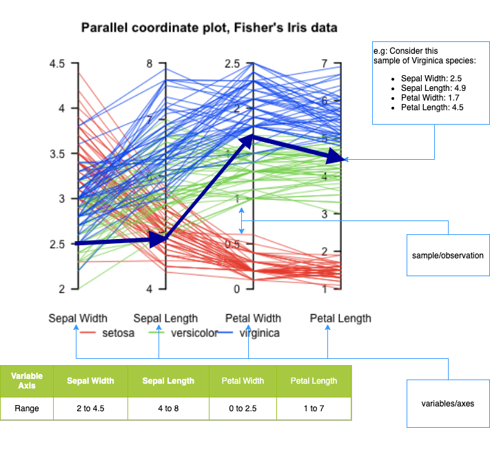
What it is:: A visualization for multivariate data where each variable is a parallel axis, and each observation is drawn as a polyline across axes.
What it’s good for:
- Comparing many variables at once
- Identifying patterns, clusters, and outliers
- Exploring tradeoffs between dimensions
How to read it:
- Each vertical axis = one variable
- Each line = one data record
- Line crossings indicate differences in relative values
Strengths:
- Scales beyond 2–3 dimensions
- Works well with interactive filtering and highlighting
- Effective for exploratory analysis
Limitations:
- Can become cluttered with many observations
- Axis ordering strongly affects interpretability
- Less effective without interaction
Typical use cases:
- High-dimensional datasets in data science, engineering metrics, model diagnostics, and exploratory analytics
Example: Iris dataset
Here’s a useful example of a Parallel Coordinates plot, showing multivariate structure in the well-known Iris dataset — where different species form distinguishable patterns across four features (sepal/petal width/length):
Example: Parallel coordinate plots
- Parallel coordinate plots are a way to visualize multivariate data by plotting each variable on a separate axis and connecting them with lines to show relationships and patterns between the variables. These are created with
px.parallel_coordinates() - The lines tie together points in the same row in the data-frame, and the height along each respective axis shows the variables value.
import plotly.express as px
import seaborn as sns

df = sns.load_dataset("penguins")
df = df.dropna()  # drop rows with nan
print(df)

df["species"] = df.species.astype("category")
df["species_id"] = df.species.cat.codes
px.parallel_coordinates(
    df,
    color="species_id",
    color_continuous_scale=px.colors.diverging.Tealrose,
    height=300,
    width=1000,
    labels={"bill_length_mm": "Bill length (mm)"},

)
species island bill_length_mm bill_depth_mm flipper_length_mm \
0 Adelie Torgersen 39.1 18.7 181.0
1 Adelie Torgersen 39.5 17.4 186.0
2 Adelie Torgersen 40.3 18.0 195.0
4 Adelie Torgersen 36.7 19.3 193.0
5 Adelie Torgersen 39.3 20.6 190.0
.. ... ... ... ... ...
338 Gentoo Biscoe 47.2 13.7 214.0
340 Gentoo Biscoe 46.8 14.3 215.0
341 Gentoo Biscoe 50.4 15.7 222.0
342 Gentoo Biscoe 45.2 14.8 212.0
343 Gentoo Biscoe 49.9 16.1 213.0
body_mass_g sex
0 3750.0 Male
1 3800.0 Female
2 3250.0 Female
4 3450.0 Female
5 3650.0 Male
.. ... ...
338 4925.0 Female
340 4850.0 Female
341 5750.0 Male
342 5200.0 Female
343 5400.0 Male
[333 rows x 7 columns]Tree-maps
- A tree-map graph is a type of visualization that uses nested rectangles to display hierarchical data. Each rectangle represents a category, and its size corresponds to the value of that category. This is done with the
px.treemap()function
import plotly.express as px
import numpy as np

# There is no `mpg` dataset in plotly.express.data.
# We'll use the seaborn 'mpg' dataset for this example instead:
import seaborn as sns
df = sns.load_dataset("mpg").dropna()

# We'll nest the data by origin and manufacturer, and size by count (since there's no obvious "size" variable)
df["all"] = "all_cars"

# The 'mpg' dataset does not have a 'manufacturer' column; let's extract manufacturer from the 'name' (it's before the first space)
df["manufacturer"] = df["name"].apply(lambda x: x.split()[0])

mpg_counts = df.groupby(["all", "origin", "manufacturer"], as_index=False).size()
mpg_avg_mpg = df.groupby(["all", "origin", "manufacturer"], as_index=False)["mpg"].mean()
df_treemap = mpg_counts.merge(mpg_avg_mpg, on=["all", "origin", "manufacturer"], how="left")

fig = px.treemap(
    df_treemap,
    path=["all", "origin", "manufacturer"],  # hierarchical path
    values="size",                          # size (number of cars)
    color="mpg",                            # average mpg by group
    hover_data={"size":True, "mpg":":.1f"},
    color_continuous_scale="RdBu",
    color_continuous_midpoint=np.average(df["mpg"]),
    height=450
)
fig.show()
Unable to display output for mime type(s): application/vnd.plotly.v1+jsonPlotly: 3D graphs
- We can also generate graphics in 3D Cartesian space using
px.scatter_3d
# SOURCE: https://towardsdatascience.com/cheat-codes-to-better-
# visualisations-with-plotly-express-21caece3db01

import plotly.express as px
import seaborn as sns

# GET DATA
election = px.data.election()

# GENERATE FIGURE
fig = px.scatter_3d(
    election,  # dataframe
    x="Joly",  # x-values column
    y="Coderre",  # y-values column
    z="Bergeron",  # z-values column
    color="winner",  # column shown by color
    width=900,
    height=600,
    hover_name="district",  # hover title
    symbol="result",  # column shown by shape
    color_discrete_map={"Joly": "blue", "Bergeron": "green", "Coderre": "red"},
)
# specific colors for x,y,z values            )
fig.show()
Keep Geometry in “check”
Plotly Express automatically applies a square-root scaling to bubble sizes.
Specifically:
- When you pass a column to
size=in functions likepx.scatter, Plotly Express maps the data values to marker area, not radius. - Internally, this means the radius is proportional to √(value), so perceived bubble area matches the data.
This is intentional and aligns with visualization best practices, since humans perceive area, not radius.
If you want direct control, you can:
- Pre-transform the data yourself, or
- Use Graph Objects and explicitly set
marker.sizeandmarker.sizeref.
Key takeaway: Plotly Express does the perceptually correct thing by default for bubble plots.
import plotly.express as px

# Define the data
x = [1, 2, 3, 4]
y = [1, 2, 3, 4]
sizes = [20, 40, 80, 160]

fig = px.scatter(
    x=x,
    y=y,
    size=sizes,
    size_max=160,
    title="Simple Bubble Plot",
    labels={'x': 'X Value', 'y': 'Y Value'},
)

fig.show()
Unable to display output for mime type(s): application/vnd.plotly.v1+jsonimport plotly.express as px
import numpy as np
# Define the data
x = [1, 2, 3, 4]
y = [1, 2, 3, 4]
sizes = np.array([20, 40, 80, 160])**0.5
fig = px.scatter(
x=x,
y=y,
size=sizes,
size_max=160,
title="Simple Bubble Plot",
labels={'x': 'X Value', 'y': 'Y Value'},
)
fig.show()Unable to display output for mime type(s): application/vnd.plotly.v1+jsonExample: Plotly themes
- Plotly has various built in themes, similar to MPL and GGPLOT.
- The following code demonstrates the various themes with the Gap-minder dataset
# https://plotly.com/python/templates/
import plotly.express as px

df = px.data.gapminder()
df_2007 = df.query("year==2007")
k = 0
for template in [
    "plotly",
    "plotly_white",
    "plotly_dark",
    "ggplot2",
    "seaborn",
    "none",
    "simple_white",
]:
    fig = px.scatter(
        df_2007,
        x="gdpPercap",
        y="lifeExp",
        size=df_2007["pop"],
        color="continent",
        log_x=True,
        size_max=60,
        template=template,
        title="Gapminder 2007: '%s' theme" % template,
    )

    file_name = "./img/plotly-theme-" + str(k) + ".html"
    # print(file_name)
    fig.write_html(file_name)
    fig.show()
    k += 1

# from IPython.display import IFrame
# IFrame(src=file_name, width=1000, height=500)
Facets
- Of course we also often want to include subplots through faceting. This is done using the
facet_colandfacet_col_wrapcommands - As mentioned above, combining figures objects into subplots requires
plotly.go
import plotly.express as px

# import seaborn as sns

gap = px.data.gapminder()
fig = px.line(
    data_frame=gap,
    x="year",
    y="lifeExp",
    color="continent",
    facet_col="continent",
    # line_group="country",
    facet_col_wrap=3,  # << facet_col is the key
    labels={"lifeExp": "Life expectancy"},  # , "year" : 'Time (years)'},
    template="plotly_white",
    width=1000,
    height=1000,
).update_layout(showlegend=False)
fig.show()
Customization the tool-tip
- We can modify the hover options using the following command
import plotly.express as px
import seaborn as sns

df = sns.load_dataset("penguins")
df = df.dropna()  # drop rows with nan

fig = px.scatter(
    data_frame=df,
    x="bill_length_mm",
    y="body_mass_g",
    size=df["flipper_length_mm"],
    color="species",
    template="plotly_white",
    labels={
        "bill_length_mm": "Bill length (mm)",
        "body_mass_g": "Body mass (g)",
        "species": "Species",
    },
    title="Palmer Penguins",
)

# UPDATE TOOL TIP
fig.update_traces(
    customdata=df,
    hovertemplate="Island: %{customdata[1]} <br>Sex: %{customdata[6]}",
)

fig.show()
Animation and sliders
Plotly provides a range of tools that makes adding animations to visualizations easy.
px.scatter(
    px.data.gapminder(),
    x="gdpPercap",
    y="lifeExp",
    animation_frame="year",
    animation_group="country",
    size="pop",
    color="continent",
    hover_name="country",
    template="plotly_white",
    log_x=True,
    size_max=45,
    range_x=[100, 100000],
    range_y=[25, 90],
)
Choropleths
- We will cover
Choroplethsin more detail during theGeo-spatial module. - However, for now, all you need to know is that a choropleth is a type of map that uses colors or shading to represent different values of a particular data variable across a geographic area, such as a country, state, or city.
- The choropleth map divides the area into regions or polygons, usually based on administrative boundaries, and then assigns a color or shade to each region based on the value of the data variable being represented.
- For example, if the data variable is
population density, then regions with higher density would be shaded darker than regions with lower population density.
Example: Choropleths
Plotly can internally create the map using location tags for countries, such as USA.
import plotly.express as px
import seaborn as sns

# SOURCE: https://towardsdatascience.com/cheat-codes-to-better-
# visualisations-with-plotly-express-21caece3db01

gapminder = px.data.gapminder()

fig = px.choropleth(
    gapminder,  # dataframe
    locations="iso_alpha",  # location code
    color="lifeExp",  # column shown by color
    hover_name="country",  # hover info title
    animation_frame="year",  # column animated
    range_color=[20, 80],  # color range
)
fig.show()
More Advanced: Plotly.py
Graph objects
Note: Graph objects are covered heavily in the lab, so we only introduce the fundamentals here
Motivation
- As we have seen, using
Plotly expressis generally easy and straight-forward. - However, when you want to increase the complexity of a graph, you often need to switch to
plotly graph objectsand things can get quite involved. - Understanding Graph objects gives you FULL customization control over your graphs
- For example, sliders, maps, and drop-down menus are easy individually with
Plotly express, however combining them withplotly graph objectsis non-trivial.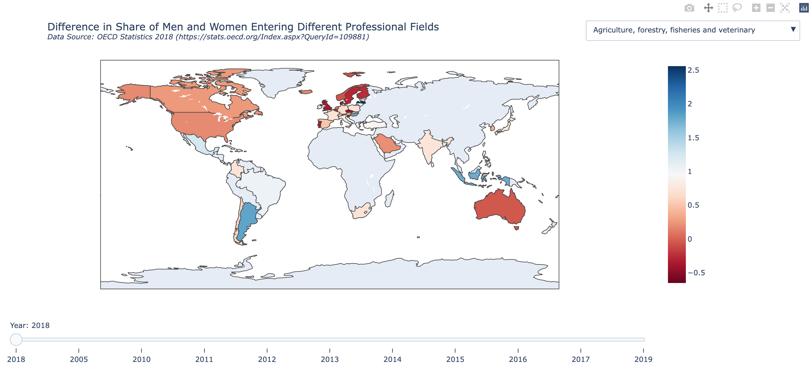
- Click here for interactive version of the map example
Plotly Graph Objects overview
- What Graph Objects Are
- Low-level, explicit API in Plotly
- Direct mapping to Plotly.js figure schema
- Figure–Trace–Layout Model
Figureas container- Traces as visual layers
- Layout as global configuration
- Creating Traces
- Common trace types (
Scatter,Bar,Heatmap, etc.) - Supplying data arrays
- Marker, line, and text properties
- Common trace types (
- Layout Control
- Axes, titles, legends
- Annotations and shapes
- Margins, sizing, templates
- Updating Figures
add_trace,update_traces,update_layout- Chaining and partial updates
- Subplots
- Creating multi-panel figures
- Shared vs independent axes
- Interactivity
- Hover behavior
- Selections and legend interactions
- Performance & Rendering
- SVG vs WebGL traces
- When to switch (
Scattergl, etc.)
- When to Use Graph Objects
- Fine-grained control
- Complex layouts
- When Plotly Express is insufficient
Structure of a graph object
Plotly figuresare represented as hierarchical trees, withGraph_objectsbeing the root note, and child-nodes calledattributes.- Graph_objects have three top-level attributes:
data,layout, andframes(frames are only needed for animated plots)- Notice the connection of these attributes to pure
JavaScriptmentioned earlier.
- Notice the connection of these attributes to pure
- Data: This is a list of dictionaries referred to as “traces”
- The
tracerepresents a set of related graphical marks in a figure. - Each trace must have a
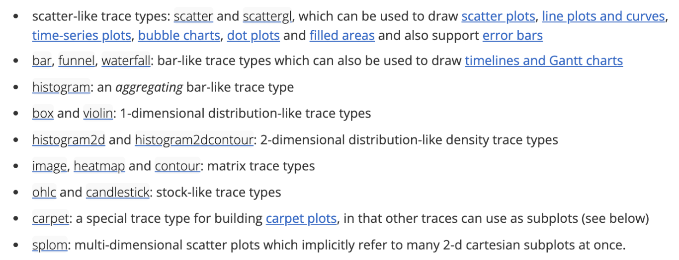
typeattribute which defines the other allowable attributes. - Each trace has one of more than 40 possible types (see below for a list organized by subplot type, including e.g.
scatter,bar,pie,surface,choroplethetc)
- The
- Layout: Controls various structural and stylistic components (e.g. title, font, size, etc)
Sources: figure structure Graph objects
Graph_object Structure summary
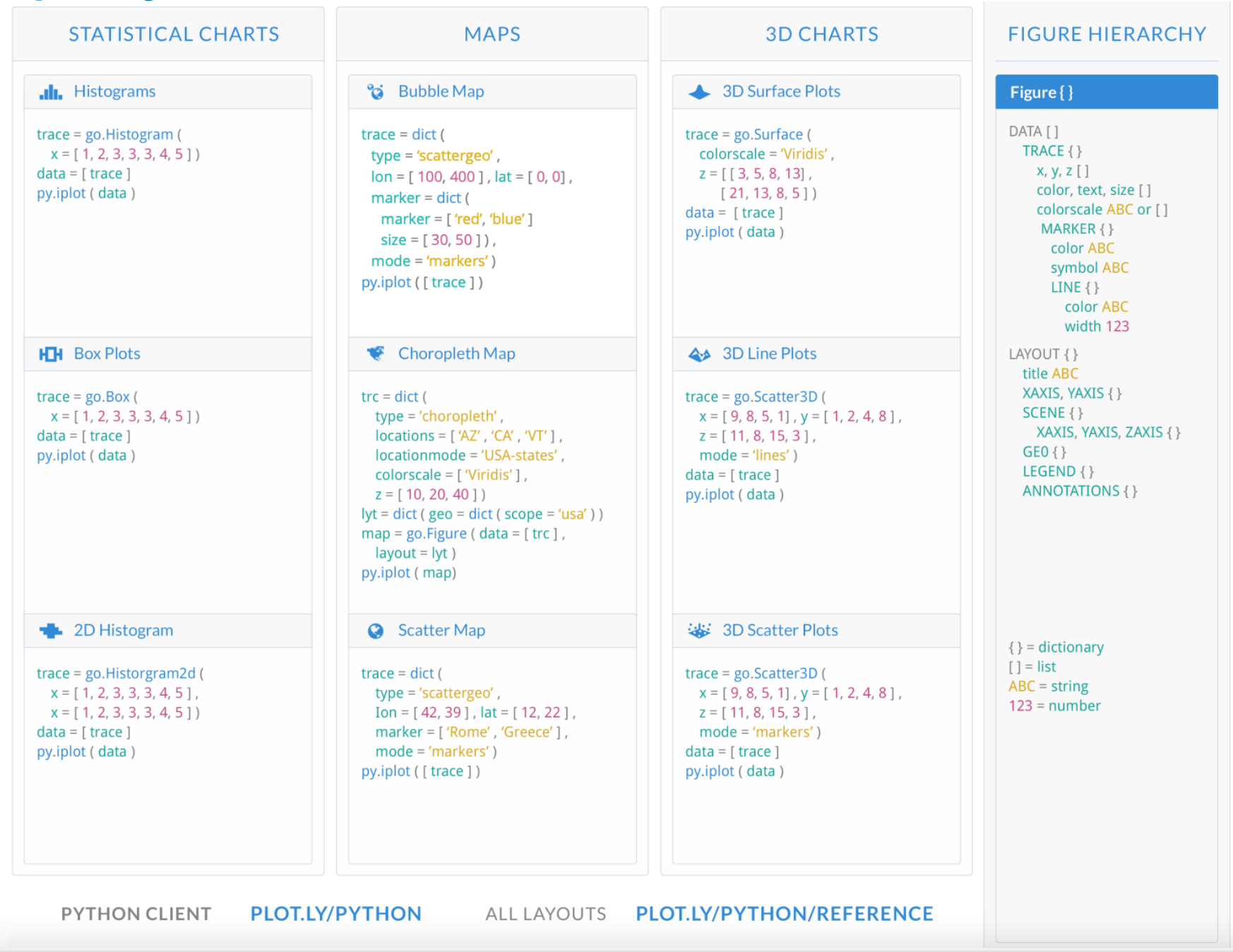
Various available traces
- 2D Cartesian trace types, and Subplots.
- Geo-spatial trace Types.
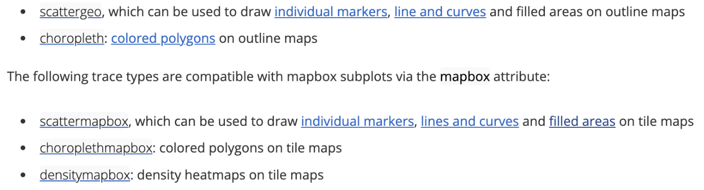
For more click here!
Looking under the hood
- Viewing the underlying data structure for any plotly.graph_objects.Figure object can be done via print(fig) or fig.show(“json”).
- Figures also support fig.to_dict() and fig.to_json() methods.
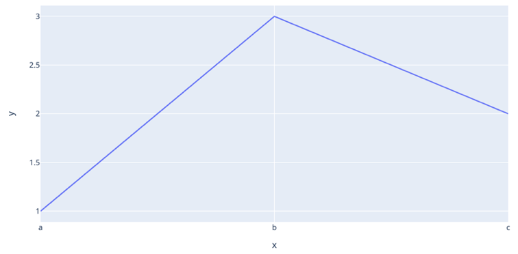
import plotly.express as px

fig = px.line(x=["a", "b", "c"], y=[1, 3, 2], title="sample figure")
print(fig)
# fig.show()
Figure({
'data': [{'hovertemplate': 'x=%{x}<br>y=%{y}<extra></extra>',
'legendgroup': '',
'line': {'color': '#636efa', 'dash': 'solid'},
'marker': {'symbol': 'circle'},
'mode': 'lines',
'name': '',
'orientation': 'v',
'showlegend': False,
'type': 'scatter',
'x': array(['a', 'b', 'c'], dtype=object),
'xaxis': 'x',
'y': {'bdata': 'AQMC', 'dtype': 'i1'},
'yaxis': 'y'}],
'layout': {'legend': {'tracegroupgap': 0},
'template': '...',
'title': {'text': 'sample figure'},
'xaxis': {'anchor': 'y', 'domain': [0.0, 1.0], 'title': {'text': 'x'}},
'yaxis': {'anchor': 'x', 'domain': [0.0, 1.0], 'title': {'text': 'y'}}}
})Graph_objects: Hello world
- When using graph objects (without animation), you typically do the following
(1)Initialize the figure(2)Add one or more traces(3)customize the layout
import plotly.express as px
import plotly.graph_objects as go

# DATAFRAME
df = px.data.gapminder()

# INITIALIZE GRAPH OBJECT
fig = go.Figure()

# ADD TRACES FOR THE DATA-FRAME
fig.add_trace(
    go.Scatter(
        x=df["gdpPercap"],
        y=df["lifeExp"],
        mode="markers",
        # Note: marker expects a dictionary, so use {} not dict()
        marker={
            "size": 50 * (df["pop"] / df["pop"].max()) ** 0.5,
            "color": df["pop"],
            "showscale": True,
            "colorscale": "Viridis",
            "symbol": "circle",
        },
        opacity=1.0,
    )
)

# SET THEME, AXIS LABELS, AND LOG SCALE
fig.update_layout(
    template="plotly_white",
    xaxis_title="National GDP (per capita)",
    yaxis_title="Life expectancy (years)",
    title="Country comparison: color & size = population",
    height=400,
    width=800,
)
fig.update_xaxes(type="log")

fig.show()
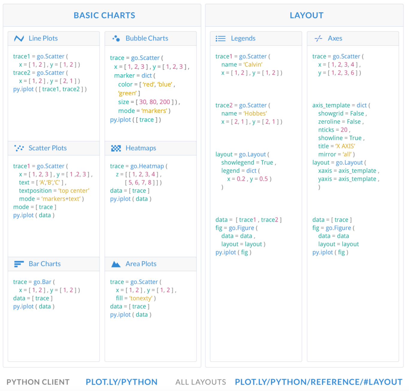
Basic charts with graph_objects
Additional charts with Graph objects
Subplots
With plotly.graph_objects we can finally combine figures in a subplot! source
from plotly.subplots import make_subplots
import plotly.graph_objects as go

fig = make_subplots(rows=1, cols=2)

fig.add_trace(
    go.Scatter(x=[1, 2, 3], y=[4, 5, 6]),
    row=1, col=1
)

fig.add_trace(
    go.Scatter(x=[20, 30, 40], y=[50, 60, 70]),
    row=1, col=2
)

fig.update_layout(height=500, width=700, title_text="Side By Side Subplots")
fig.show()
Multiple Subplots
Here we show a 2 x 2 subplot grid with each subplot populated with a single scatter trace.
import plotly.graph_objects as go
from plotly.subplots import make_subplots

fig = make_subplots(rows=2, cols=2, start_cell="bottom-left")

fig.add_trace(go.Scatter(x=[1, 2, 3], y=[4, 5, 6]),
              row=1, col=1)

fig.add_trace(go.Scatter(x=[20, 30, 40], y=[50, 60, 70]),
              row=1, col=2)

fig.add_trace(go.Scatter(x=[300, 400, 500], y=[600, 700, 800]),
              row=2, col=1)

fig.add_trace(go.Scatter(x=[4000, 5000, 6000], y=[7000, 8000, 9000]),
              row=2, col=2)

fig.show()
Sliders in Plotly Graph Objects
What they are: Layout-level UI controls (
layout.sliders) made of discrete steps that update figure state.What they do: Select among predefined states by updating trace visibility, data, or layout — no dynamic computation.
Common pattern (masking):
- One trace per slider value (state)
- Slider steps toggle
visiblemasks to show the active trace(s)
Alternative pattern (animations):
- Fixed set of traces
- Slider steps through frames that update trace data
Rule of thumb:
- Independent states → one trace per state + visibility masks
- Sequential states (e.g., time) → frames + slider
SVG vs WebGL Traces in Plotly
SVG Traces
- DOM-based rendering using SVG elements
- Best for small to medium datasets
- High visual precision (text, annotations, crisp lines)
- Easier to style and export (PDF, SVG)
WebGL Traces
- GPU-accelerated rendering via WebGL
- Designed for large datasets (10⁴–10⁶+ points)
- Faster interaction (pan, zoom) at scale
- Limited styling and export fidelity
Rule of thumb: Use SVG for publication-quality visuals and WebGL when performance with large data matters.
How to Switch Between SVG and WebGL in Plotly
You switch by choosing the trace type (not a global flag).
In Python
- SVG (default):
go.Scatter(x=x, y=y)- WebGL:
go.Scattergl(x=x, y=y)Other common WebGL variants:
go.Pointcloudgo.Heatmapgl
In R
- SVG (default):
plot_ly(x = x, y = y, type = "scatter", mode = "markers")- WebGL:
plot_ly(x = x, y = y, type = "scattergl", mode = "markers")Plotly Express (Python)
- SVG (default):
px.scatter(df, x="x", y="y")- WebGL:
px.scatter(df, x="x", y="y", render_mode="webgl")Key point: SVG vs WebGL is a trace-level decision—use WebGL (*gl traces) when performance matters, SVG otherwise.
from plotly.subplots import make_subplots
import plotly.graph_objects as go

fig = go.Figure()

N=100000
x=np.random.randn(N)
y=2*x+np.random.randn(N)
fig.add_trace(go.Scattergl(x=x, y=y, mode="markers"))
# fig.add_trace(go.Scatter(x=x, y=y, mode="markers"))

fig.update_layout(height=500, width=700, title_text="Side By Side Subplots")
fig.show()
Resources
- Graph objects are covered heavily in the lab, so we only introduced the basics here
- Also the documentation on the Plotly website is very good: https://plotly.com/python/
- This provides a massive collection of examples, for both
plotly-expressandgraph-objects, which can get you started on almost any task.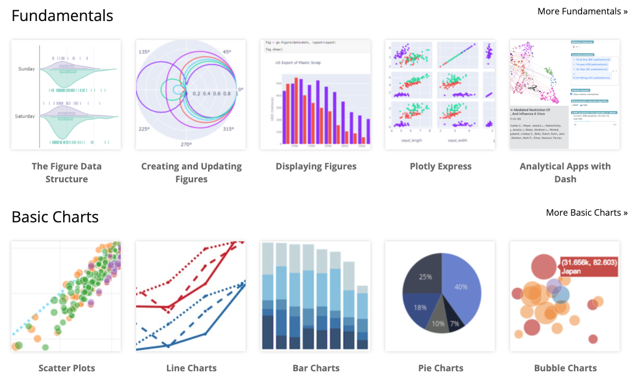
Plot digitizers
Optional: additional content
Overview
- This is un-related to Plotly, however,
plot digitizersare a useful tool for extracting theraw numeric datafrom plots quickly - Web plot digitizer is a free online tool for doing this
- Important: This process isn’t perfect, so use extra care, results should be double-checked, and the process documented. Especially when results are consequential. Furthermore, digitized results may not be suitable for academic publications.
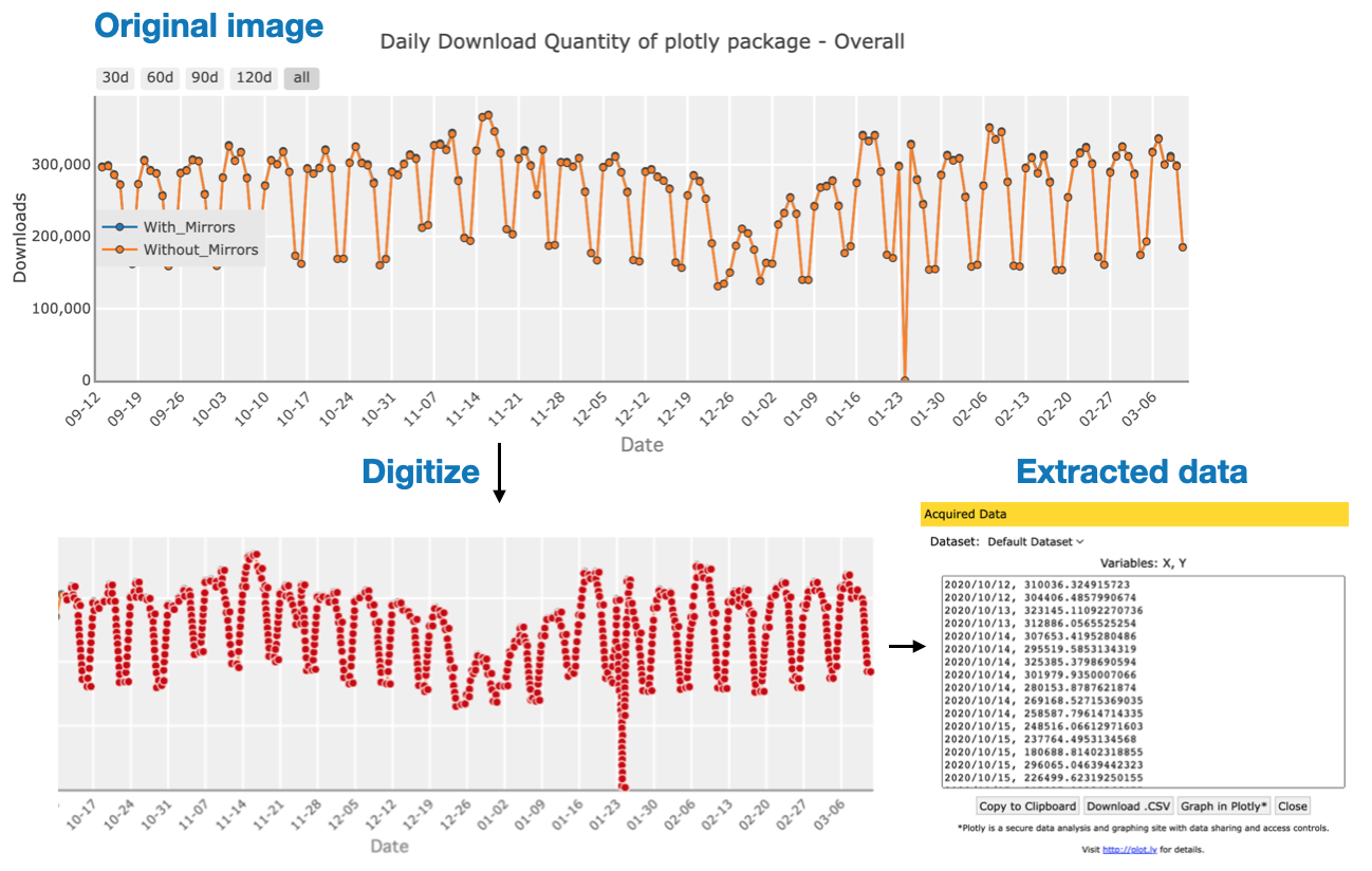
Digitization process:
- Upload image.
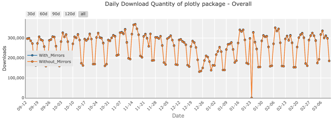
- Upload image.
- Define coordinate axis.
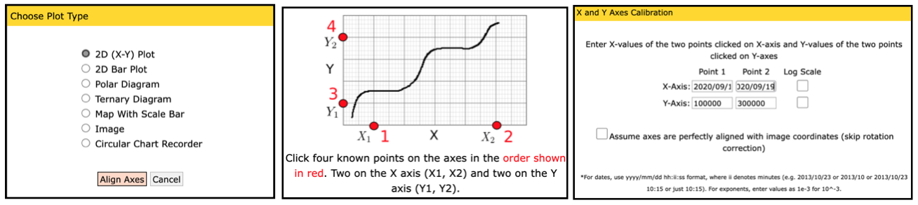
- Define coordinate axis.
Digitization process:
- Digitize: Either manually or using the automated method
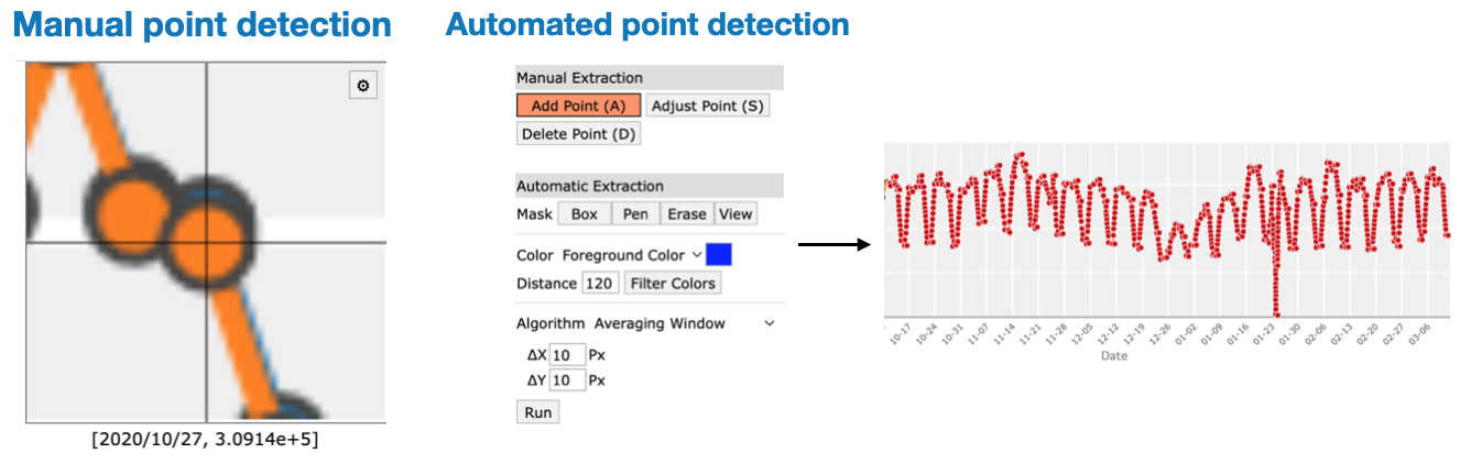
- Digitize: Either manually or using the automated method
- Export data: Either to a file or export automatically to
Plotly chart-studio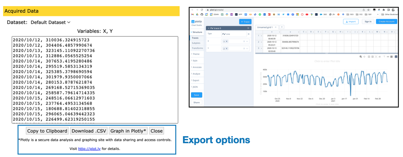
- Export data: Either to a file or export automatically to