import numpy as np
import pandas as pd
import matplotlib.pyplot as plt
import seaborn as sns

sns.set_theme()                      # default Seaborn theme
print("seaborn", sns.__version__)
seaborn 0.13.2x, y, hue, size, style, col, row)sns, plt, pd, npsns.set_theme() applies Seaborn’s default look to every plot that followsimport numpy as np
import pandas as pd
import matplotlib.pyplot as plt
import seaborn as sns
sns.set_theme() # default Seaborn theme
print("seaborn", sns.__version__)seaborn 0.13.2country, continent, year, lifeExp (years), pop (people), gdpPercap (inflation-adjusted USD)plotly.express.data.gapminder() returns the same tableurl = "https://raw.githubusercontent.com/plotly/datasets/master/gapminderDataFiveYear.csv"
gm_raw = pd.read_csv(url)
gm_raw.head()| country | year | pop | continent | lifeExp | gdpPercap | |
|---|---|---|---|---|---|---|
| 0 | Afghanistan | 1952 | 8425333.0 | Asia | 28.801 | 779.445314 |
| 1 | Afghanistan | 1957 | 9240934.0 | Asia | 30.332 | 820.853030 |
| 2 | Afghanistan | 1962 | 10267083.0 | Asia | 31.997 | 853.100710 |
| 3 | Afghanistan | 1967 | 11537966.0 | Asia | 34.020 | 836.197138 |
| 4 | Afghanistan | 1972 | 13079460.0 | Asia | 36.088 | 739.981106 |
info() gives all three at onceprint(gm_raw.shape)
gm_raw.info()(1704, 6)
<class 'pandas.core.frame.DataFrame'>
RangeIndex: 1704 entries, 0 to 1703
Data columns (total 6 columns):
# Column Non-Null Count Dtype
--- ------ -------------- -----
0 country 1704 non-null object
1 year 1704 non-null int64
2 pop 1704 non-null float64
3 continent 1704 non-null object
4 lifeExp 1704 non-null float64
5 gdpPercap 1704 non-null float64
dtypes: float64(3), int64(1), object(2)
memory usage: 80.0+ KBprint("Missing values:", gm_raw.isna().sum().sum())
print("Duplicate rows:", gm_raw.duplicated().sum())
print("Countries:", gm_raw["country"].nunique(), "| Years:", sorted(gm_raw["year"].unique()))Missing values: 0
Duplicate rows: 0
Countries: 142 | Years: [np.int64(1952), np.int64(1957), np.int64(1962), np.int64(1967), np.int64(1972), np.int64(1977), np.int64(1982), np.int64(1987), np.int64(1992), np.int64(1997), np.int64(2002), np.int64(2007)]describe() for numeric columns; value_counts() for categoriespop and gdpPercap span several orders of magnitude (a hint that log scales will help)gm_raw.describe().round(1)| year | pop | lifeExp | gdpPercap | |
|---|---|---|---|---|
| count | 1704.0 | 1.704000e+03 | 1704.0 | 1704.0 |
| mean | 1979.5 | 2.960121e+07 | 59.5 | 7215.3 |
| std | 17.3 | 1.061579e+08 | 12.9 | 9857.5 |
| min | 1952.0 | 6.001100e+04 | 23.6 | 241.2 |
| 25% | 1965.8 | 2.793664e+06 | 48.2 | 1202.1 |
| 50% | 1979.5 | 7.023596e+06 | 60.7 | 3531.8 |
| 75% | 1993.2 | 1.958522e+07 | 70.8 | 9325.5 |
| max | 2007.0 | 1.318683e+09 | 82.6 | 113523.1 |
gm_raw.drop_duplicates("country")["continent"].value_counts() # countries per continentcontinent
Africa 52
Asia 33
Europe 30
Americas 25
Oceania 2
Name: count, dtype: int64snake_casecontinent an ordered categorical so every plot uses the same order and colorsgm = gm_raw.rename(columns={"lifeExp": "life_exp", "gdpPercap": "gdp_per_cap"})
continent_order = ["Africa", "Americas", "Asia", "Europe", "Oceania"]
gm["continent"] = pd.Categorical(gm["continent"], categories=continent_order, ordered=True)
gm["pop_m"] = gm["pop"] / 1e6 # population in millions
gm["log_gdp"] = np.log10(gm["gdp_per_cap"]) # log10 GDP per capita
gm.head()| country | year | pop | continent | life_exp | gdp_per_cap | pop_m | log_gdp | |
|---|---|---|---|---|---|---|---|---|
| 0 | Afghanistan | 1952 | 8425333.0 | Asia | 28.801 | 779.445314 | 8.425333 | 2.891786 |
| 1 | Afghanistan | 1957 | 9240934.0 | Asia | 30.332 | 820.853030 | 9.240934 | 2.914265 |
| 2 | Afghanistan | 1962 | 10267083.0 | Asia | 31.997 | 853.100710 | 10.267083 | 2.931000 |
| 3 | Afghanistan | 1967 | 11537966.0 | Asia | 34.020 | 836.197138 | 11.537966 | 2.922309 |
| 4 | Afghanistan | 1972 | 13079460.0 | Asia | 36.088 | 739.981106 | 13.079460 | 2.869221 |
gm07 for cross-sectional plots and the full gm for trends over timegm07 = gm[gm["year"] == 2007].copy()
print(gm07.shape)
gm07.sort_values("life_exp").head(3)(142, 8)| country | year | pop | continent | life_exp | gdp_per_cap | pop_m | log_gdp | |
|---|---|---|---|---|---|---|---|---|
| 1463 | Swaziland | 2007 | 1133066.0 | Africa | 39.613 | 4513.480643 | 1.133066 | 3.654512 |
| 1043 | Mozambique | 2007 | 19951656.0 | Africa | 42.082 | 823.685621 | 19.951656 | 2.915761 |
| 1691 | Zambia | 2007 | 11746035.0 | Africa | 42.384 | 1271.211593 | 11.746035 | 3.104218 |
Axes: histplot, kdeplot, boxplot, scatterplot, …displot, catplot, relplothistplot, kdeplot, ecdfplot → displotcountplot, barplot, boxplot, violinplot, stripplot → catplotscatterplot, lineplot → relplotsns.func(data=df, x="col", y="col", hue="col")histplot bins one numeric variable and counts observations per binsns.histplot(data=gm07, x="life_exp")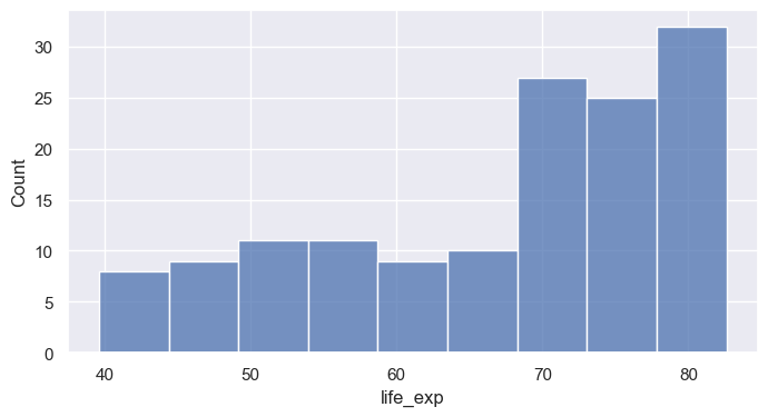
bins= sets number of bins; binwidth= sets their width (often more interpretable)stat= changes the y-axis: "count", "percent", "density", "probability"kde=True overlays a smooth density estimatesns.histplot(data=gm07, x="life_exp", binwidth=5, stat="percent", kde=True)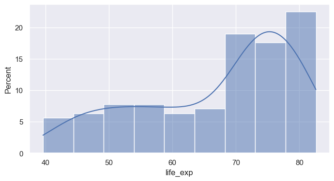
huehue= maps a categorical column to colormultiple= controls overlap: "layer" (default), "stack", "dodge", "fill"sns.histplot(data=gm07, x="life_exp", hue="continent", multiple="stack", binwidth=5)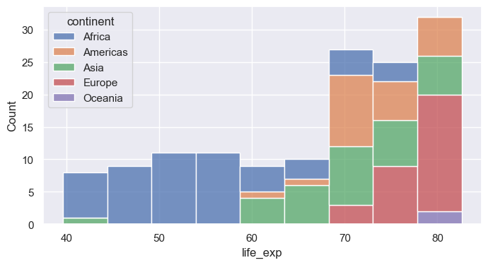
Caption: In a stacked histogram, each bar’s total height represents the total number of observations for that bin, with each color stacked on top of the previous one. For example, the blue bars at the top do not show large counts on their own—they are added above the other colors, so a short blue bar still means a small number, even if it’s high up on the plot.
sns.histplot(data=gm07, x="life_exp", hue="continent", multiple="fill", binwidth=5, alpha=0.5)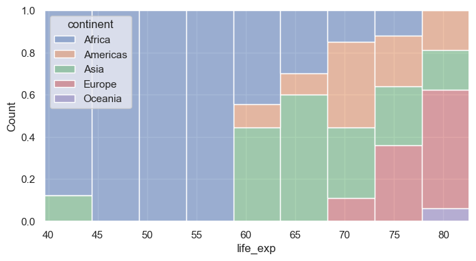
sns.histplot(data=gm07, x="life_exp", hue="continent", multiple="dodge", binwidth=5, alpha=0.5)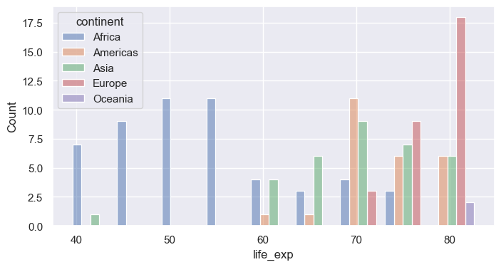
kdeplot draws a smoothed estimate of the distributionfill=True shades the area; common_norm=False normalizes each group separatelybw_adjust= controls smoothness (smaller = wigglier)sns.kdeplot(data=gm07, x="life_exp", hue="continent", fill=True, common_norm=True, alpha=0.3)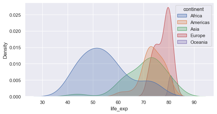
sns.kdeplot(data=gm07, x="life_exp", hue="continent", fill=True, common_norm=False, alpha=0.3)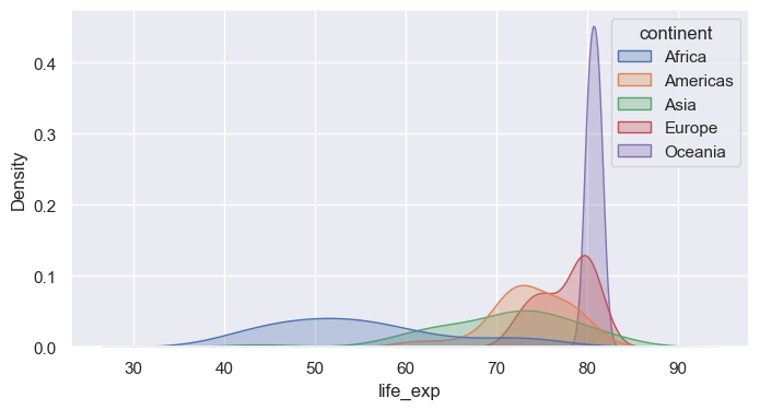
log_scale=True bins on a log axis, revealing structure hidden in the raw scalesns.histplot(data=gm07, x="gdp_per_cap")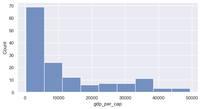
sns.histplot(data=gm07, x="gdp_per_cap", log_scale=True)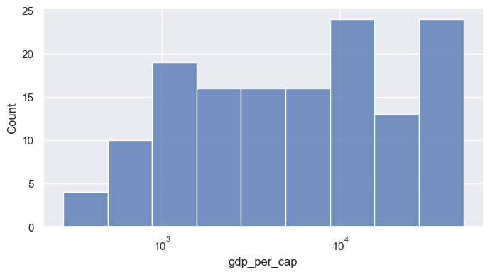
ecdfplot shows the fraction of observations at or below each valuesns.kdeplot(data=gm07, x="life_exp", hue="continent", fill=True, common_norm=False, alpha=0.3)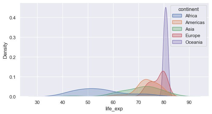
sns.ecdfplot(data=gm07, x="life_exp", hue="continent")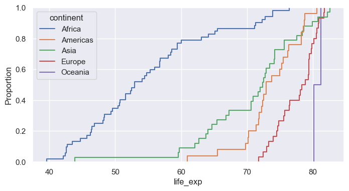
displotdisplot wraps histplot, kdeplot, ecdfplot (choose with kind=)col= and row= create small multiples, one panel per categorycol_wrap= wraps panels onto multiple rows; height= / aspect= size each panelsns.displot(data=gm07, x="life_exp", col="continent", col_wrap=3, binwidth=5, height=2.5)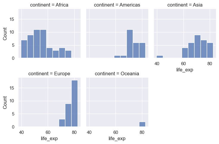
countplotsns.countplot(data=gm07, x="continent")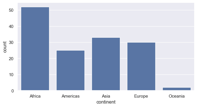
x and y for horizontal boxes (often easier to read with long labels)sns.boxplot(data=gm07, x="life_exp", y="continent")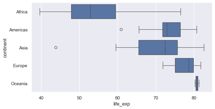
inner="quart" draws quartile lines; inner="point" shows observationscut=0 stops the density at the data rangesns.violinplot(data=gm07, x="life_exp", y="continent", inner="quart", cut=0)
plt.show() 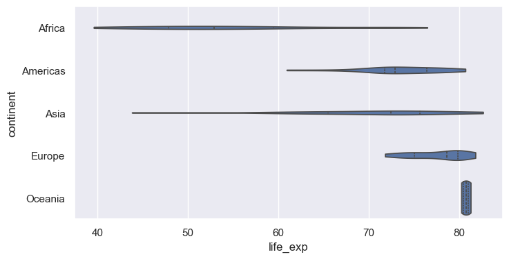
stripplot plots each point with random jitterswarmplot arranges points so none overlap (best for small to medium n)sns.boxplot(data=gm07, x="life_exp", y="continent", color="white", fliersize=0)
sns.stripplot(data=gm07, x="life_exp", y="continent", alpha=0.6)
plt.show()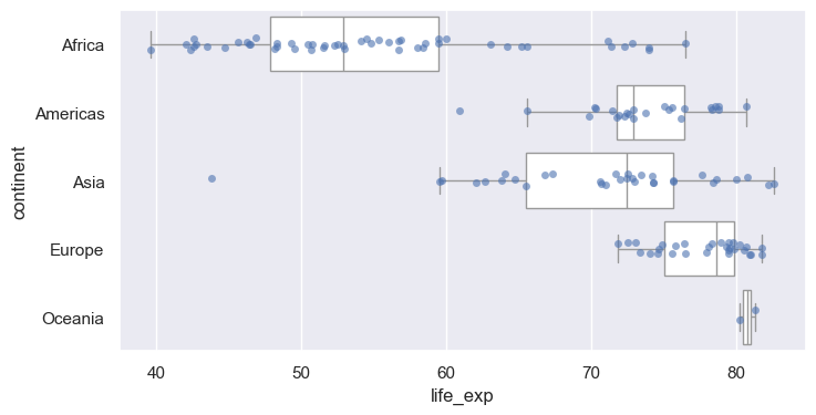
barplot computes a statistic per group (default: mean) with an error barestimator= changes the statistic (e.g., "median", "sum")errorbar= controls the interval: ("ci", 95), "sd", "se", or Nonesns.barplot(data=gm07, x="continent", y="pop_m", estimator="mean", errorbar=None)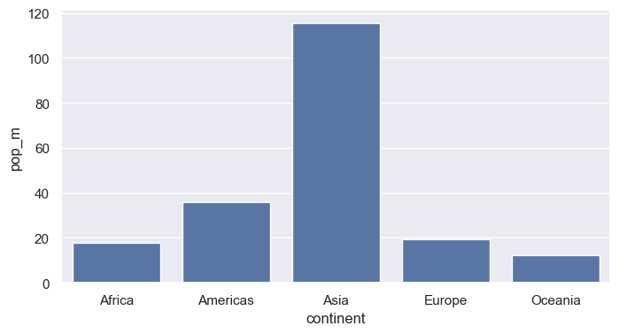
AxesAxes it drew onset_title, set_xlabel, axvline, annotate, …ax = sns.histplot(data=gm07, x="life_exp", binwidth=5)
ax.annotate("Maximum peak", xy=(65, 30), xytext=(65, 30), fontsize=12)
print(type(ax))
print(type(ax.figure))<class 'matplotlib.axes._axes.Axes'>
<class 'matplotlib.figure.Figure'>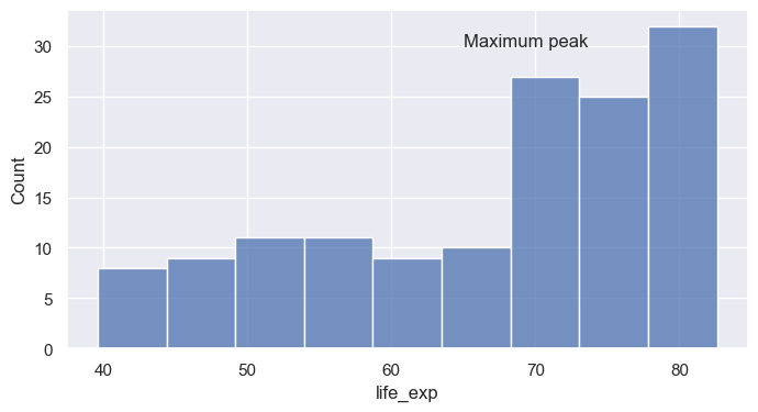
ax.set(...) sets many properties in one callax = sns.histplot(data=gm07, x="life_exp", binwidth=5)
# ax.set_title("A damped spring: the model matches the measurements", fontsize=12 + 4)
ax.set(title="Life expectancy, 2007", xlabel="Life expectancy (years)", ylabel="Number of countries", xlim=(35, 85))
FS=16
ax.title.set_fontsize(FS + 4)
ax.xaxis.label.set_fontsize(FS + 2)
ax.yaxis.label.set_fontsize(FS + 2)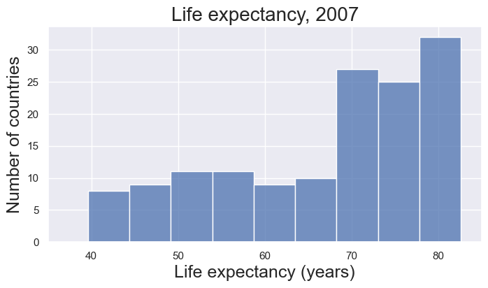
axvline / axhline add vertical or horizontal reference linesax.annotate places text with an optional arrowax = sns.histplot(data=gm07, x="life_exp", binwidth=5)
med = gm07["life_exp"].median()
ax.axvline(med, color="crimson", ls="--", lw=2)
ax.annotate(f"Median: {med:.1f} yrs", xy=(med, 25), xytext=(48, 27), arrowprops=dict(arrowstyle="->"))
ax.set(xlabel="Life expectancy (years)", ylabel="Countries")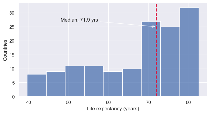
matplotlib.ticker formatters control tick label textax.tick_params adjusts size, rotation, and directionfrom matplotlib.ticker import StrMethodFormatter
ax = sns.histplot(data=gm07, x="gdp_per_cap", log_scale=True)
ax.xaxis.set_major_formatter(StrMethodFormatter("${x:,.0f}"))
ax.tick_params(axis="x", labelrotation=90)
ax.set(xlabel="GDP per capita (log scale)")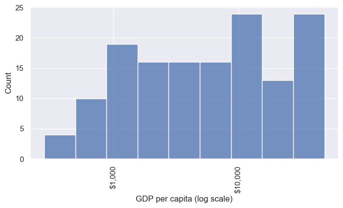
plt.subplots, then pass each Axes to Seaborn via ax=fig.suptitle adds an overall title; fig.tight_layout() fixes overlapsfig, axes = plt.subplots(1, 3, figsize=(13, 3.5))
sns.histplot(data=gm07, x="life_exp", ax=axes[0])
sns.boxplot(data=gm07, x="continent", y="life_exp", ax=axes[1])
sns.ecdfplot(data=gm07, x="gdp_per_cap", log_scale=True, ax=axes[2])
axes[1].tick_params(axis="x", labelrotation=45)
fig.suptitle("Three views of the 2007 snapshot")
fig.tight_layout()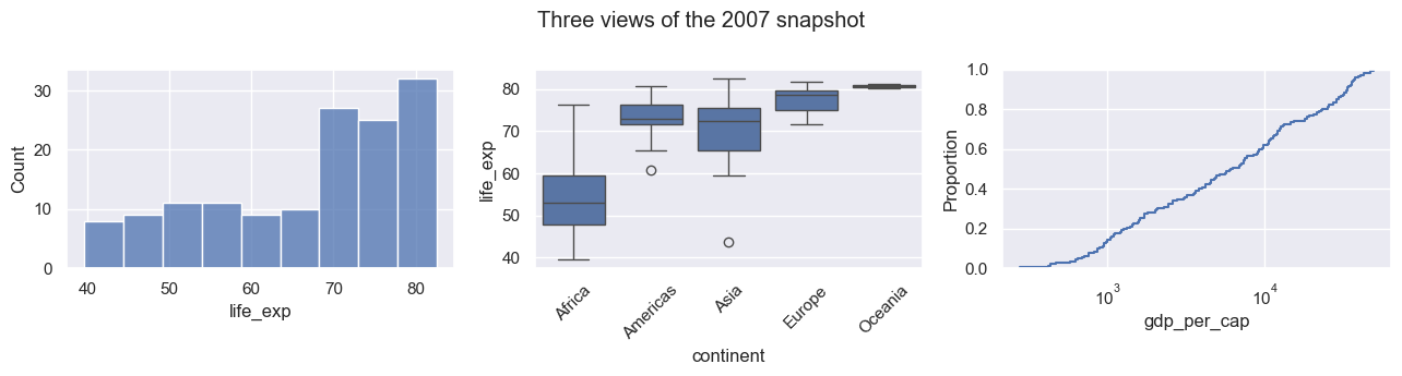
FacetGriddisplot, catplot, relplot return a grid object, not an Axesg.figure is the matplotlib Figure; g.axes is an array of Axesg.set_axis_labels, g.set_titles, g.figure.suptitleax= to figure-level functions: they create their own figureg = sns.displot(data=gm07, x="life_exp", col="continent", col_wrap=3, binwidth=5, height=2.5)
print(type(g))
g.set_axis_labels("Life expectancy (years)", "Countries")
g.set_titles("{col_name}")
g.figure.suptitle("Life expectancy by continent, 2007", y=1.03)<class 'seaborn.axisgrid.FacetGrid'>Text(0.5, 1.03, 'Life expectancy by continent, 2007')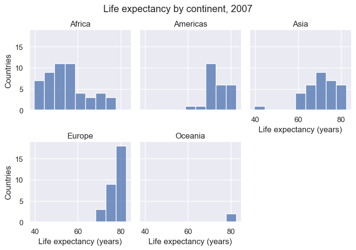
fig.savefig(...) or g.savefig(...)dpi= controls resolution; bbox_inches="tight" trims whitespace.pdf, .svg) scale cleanly in papers and slides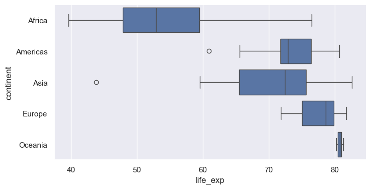
scatterplot maps one column to x and one to ysns.scatterplot(data=gm07, x="gdp_per_cap", y="life_exp")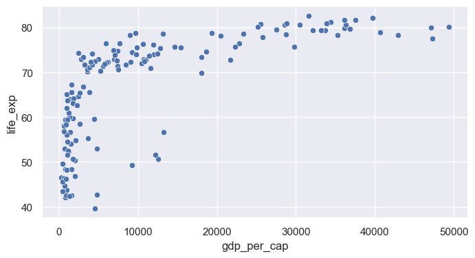
ax.set_xscale("log") (matplotlib) after plottingax = sns.scatterplot(data=gm07, x="gdp_per_cap", y="life_exp")
ax.set_xscale("log")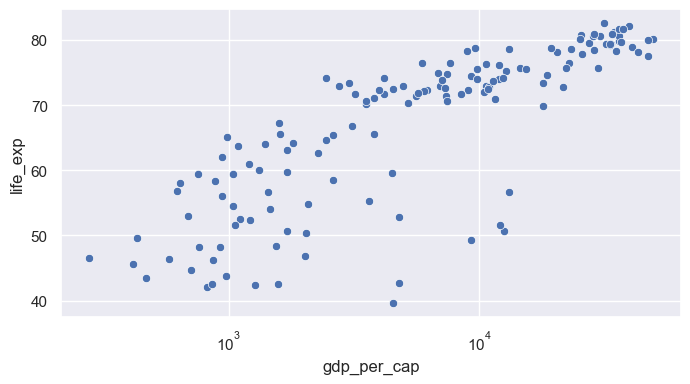
huecontinent (categorical): Seaborn chooses a qualitative palette and builds the legendax = sns.scatterplot(data=gm07, x="gdp_per_cap", y="life_exp", hue="continent")
ax.set_xscale("log")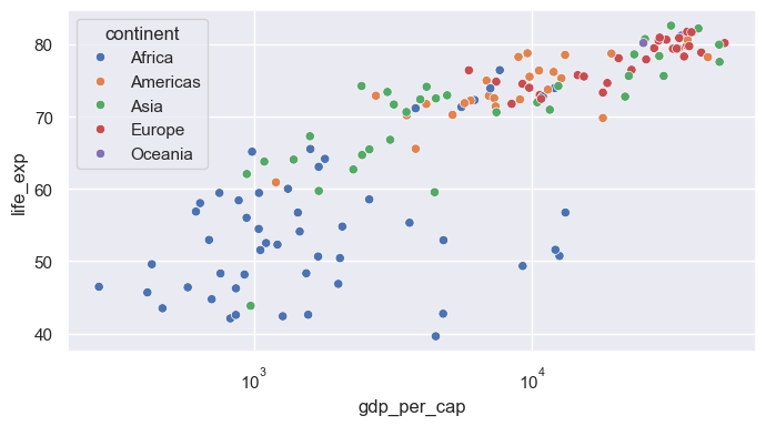
size= maps a numeric column to marker area; sizes= sets the min and max sizelegend= and bbox_to_anchor move the crowded legend outside the plotax = sns.scatterplot(data=gm07, x="gdp_per_cap", y="life_exp", hue="continent", size="pop_m",
sizes=(20, 1200), alpha=0.7, edgecolor="black")
ax.set_xscale("log")
ax.xaxis.set_major_formatter(StrMethodFormatter("${x:,.0f}"))
ax.tick_params(axis="x", labelrotation=90)
ax.set(xlabel="GDP per capita (USD, log scale)", ylabel="Life expectancy (years)", title="Wealth and health, 2007")
sns.move_legend(ax, "upper left", bbox_to_anchor=(1, 1), fontsize=8, labelspacing=1.3)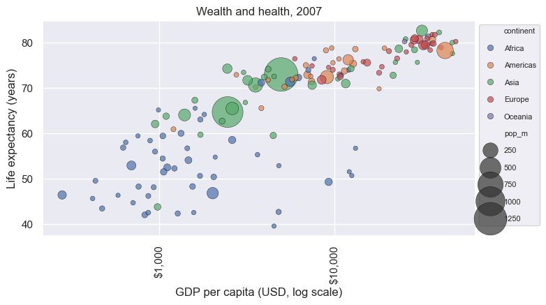
regplotregplot draws a scatter plus a linear fit with a confidence bandlogx=True fits y against log(x); lowess=True fits a flexible smooth curvescatter_kws / line_kws pass styling to each layerax = sns.regplot(data=gm07, x="gdp_per_cap", y="life_exp", logx=True,
scatter_kws={"alpha": 0.5}, line_kws={"color": "crimson"})
ax.set_xscale("log")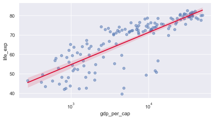
lmplotregplot: supports hue, col, rowlog_gdp column)sns.lmplot(data=gm07, x="log_gdp", y="life_exp", hue="continent", height=4, aspect=1.4, ci=None)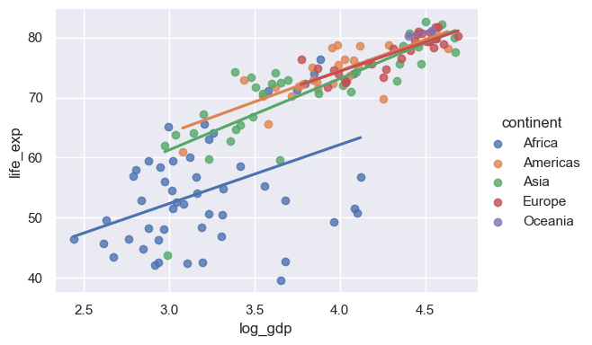
jointplotkind= options: "scatter", "kde", "hex", "reg", "hist"sns. (data=gm07, x="log_gdp", y="life_exp", hue="continent", height=5)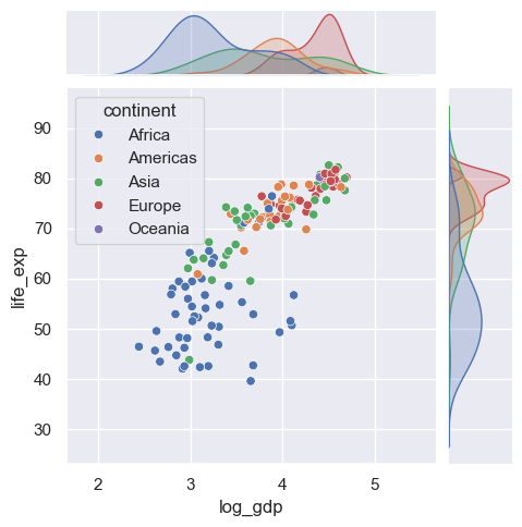
lineplotgm datax value, lineplot aggregates: plots the mean with a 95% CI bandsns.lineplot(data=gm, x="year", y="life_exp")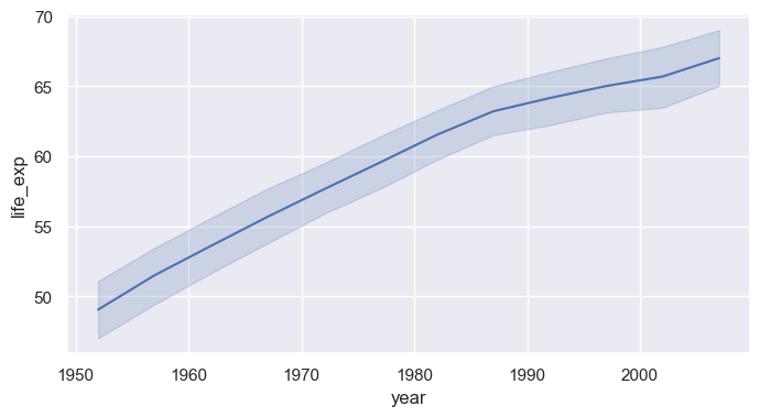
hue="continent" for one aggregated line per continenterrorbar=None removes the bands; markers=True with style= marks each observation yearsns.lineplot(data=gm, x="year", y="life_exp", hue="continent", style="continent", markers=True, dashes=False, errorbar=None)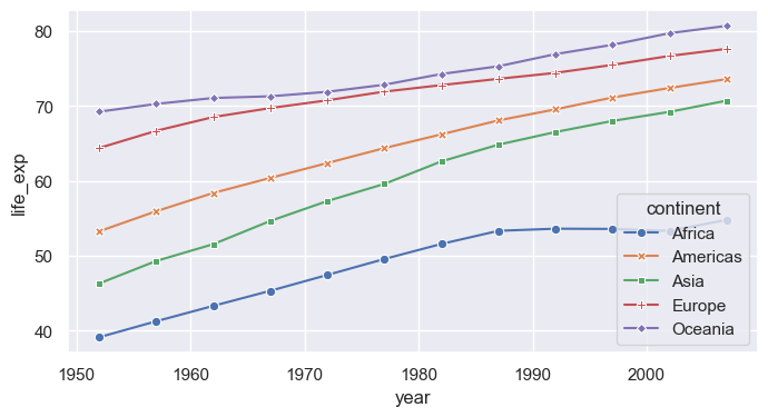
unitsunits= with estimator=None to draw each country separatelysns.lineplot(data=gm, x="year", y="life_exp", hue="continent", units="country", estimator=None, lw=0.8, alpha=0.4)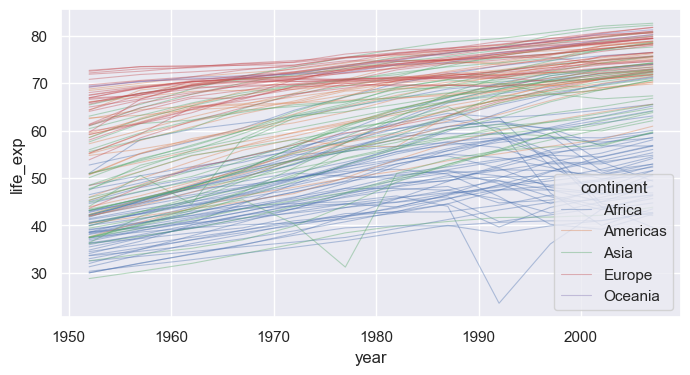
relplotscatterplot / lineplot (kind="line" or "scatter")col=, highlight a few countries on top with matplotlibg = sns.relplot(data=gm, x="year", y="life_exp", col="continent", col_wrap=3, kind="line",
units="country", estimator=None, color="gray", alpha=0.3, lw=0.8, height=2.6)
g.set_titles("{col_name}")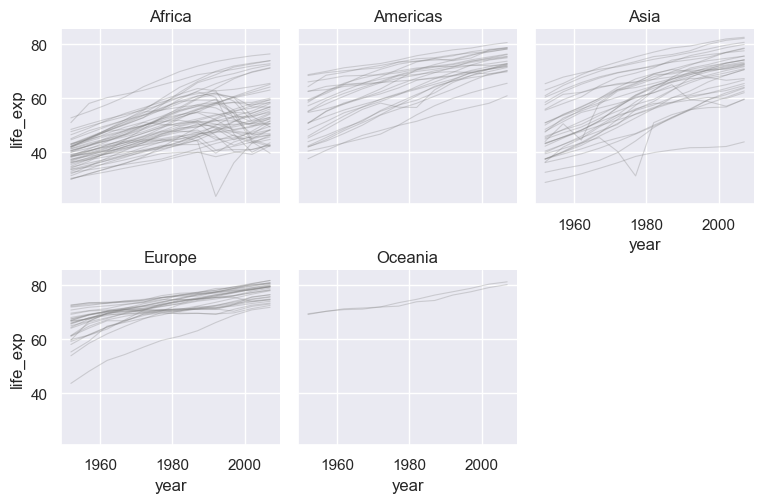
heatmap displays a 2-D table as colored cellspivot rows = country, columns = year, values = life expectancycmap= sets the colormap; annot=True would print values in each cellasia = gm[gm["continent"] == "Asia"].pivot(index="country", columns="year", values="life_exp")
asia = asia.sort_values(2007)
plt.figure(figsize=(8, 8))
sns.heatmap(asia, cmap="viridis", cbar_kws={"label": "Life expectancy (years)"})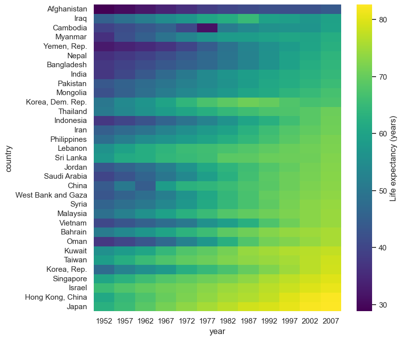
df.corr(), then heatmap with a diverging colormap centered at 0annot=True, fmt=".2f" prints each coefficientcorr = gm07[["life_exp", "gdp_per_cap", "log_gdp", "pop_m"]].corr()
sns.heatmap(corr, annot=True, fmt=".2f", cmap="vlag", center=0, vmin=-1, vmax=1, square=True)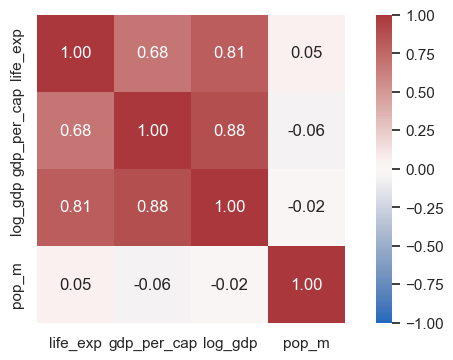
pairplotvars= selects columns; corner=True drops the redundant upper trianglesns.pairplot(data=gm07, vars=["life_exp", "log_gdp", "pop_m"], hue="continent", corner=True, height=2.3)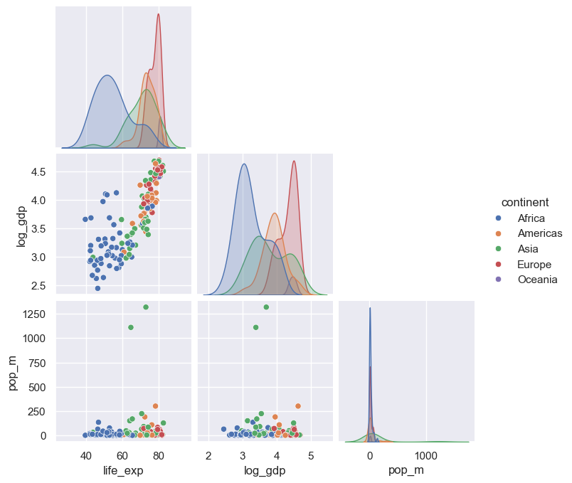
catplotkind="box", "violin", "bar", "strip", …)x (category), y (numeric), and hue (second category)years = gm[gm["year"].isin([1957, 1982, 2007])]
sns.catplot(data=years, x="continent", y="life_exp", hue="year", kind="box", height=4, aspect=1.8, palette="crest")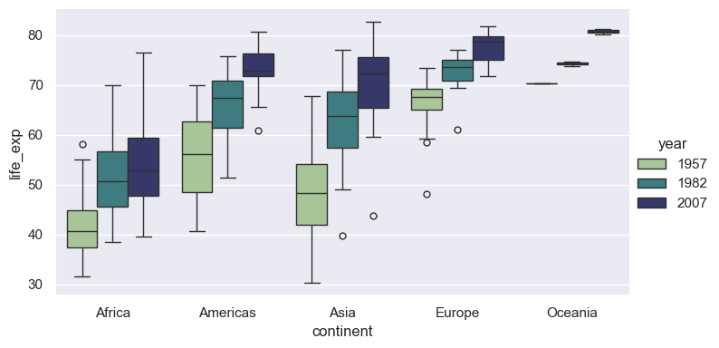
set_theme: one call for the global looksns.set_theme(style=..., context=..., palette=..., font_scale=...)darkgrid (default), whitegrid, dark, white, ticksfig = plt.figure(figsize=(16, 2.6))
for i, style in enumerate(["darkgrid", "whitegrid", "dark", "white", "ticks"]):
with sns.axes_style(style): # style applies to axes created inside the block
ax = fig.add_subplot(1, 5, i + 1)
sns.kdeplot(data=gm07, x="life_exp", fill=True, ax=ax)
ax.set(title=style, xlabel="", ylabel="", yticks=[])
fig.tight_layout()
despinewith sns.axes_style("..."): applies a style to only the plots inside the blocksns.despine() removes the top and right spines; trim=True and offset= tighten the framewhite and tickswith sns.axes_style("ticks"):
ax = sns.boxplot(data=gm07, x="life_exp", y="continent")
sns.despine(offset=8, trim=True)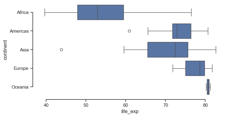
context= rescales fonts, lines, and markers for where the figure will be shown"paper" < "notebook" (default) < "talk" < "poster"font_scale= fine-tunes on top of the contextsns.set_theme(style="whitegrid", context="talk")
ax = sns.lineplot(data=gm, x="year", y="life_exp", hue="continent", errorbar=None)
sns.move_legend(ax, "upper left", bbox_to_anchor=(1, 1))
sns.set_theme() # reset to defaults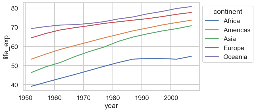
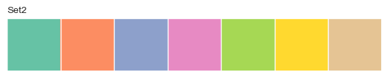
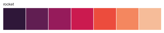
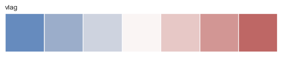
"deep" (default), "Set2", "colorblind""viridis", "rocket", "crest", "Blues""vlag", "coolwarm", "RdBu"sns.color_palette(name, n) returns a palette; sns.palplot previews itfor name in ["colorblind", "Set2", "crest", "rocket", "vlag"]:
sns.palplot(sns.color_palette(name, 7))
plt.title(name, loc="left", fontsize=10)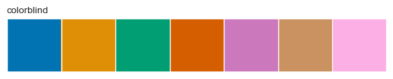

palette="name" on any function with huesns.set_palette("name") or sns.set_theme(palette="name")hue uses a continuous colormap; pass a sequential paletteax = sns.scatterplot(data=gm07, x="gdp_per_cap", y="life_exp", hue="pop_m", palette="rocket_r", hue_norm=(0, 300), size="pop_m", sizes=(10, 400))
ax.set_xscale("log")
sns.move_legend(ax, "upper left", bbox_to_anchor=(1, 1))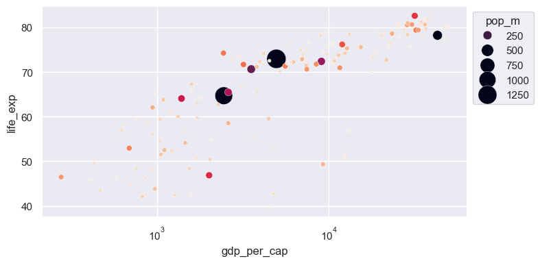
palette={category: color} to fix colors per groupcont_colors = {"Africa": "#E69F00", "Americas": "#56B4E9", "Asia": "#009E73", "Europe": "#0072B2", "Oceania": "#CC79A7"}
sns.lineplot(data=gm, x="year", y="gdp_per_cap", hue="continent", palette=cont_colors, errorbar=None)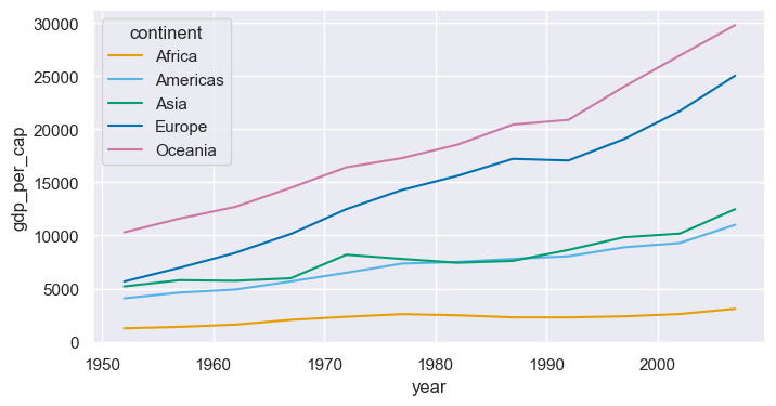
rc parametersset_theme(rc={...}) passes any matplotlib setting through Seabornplt.rcParams.keys()sns.set_theme(style="whitegrid", rc={"figure.figsize": (8, 4), "axes.spines.top": False, "axes.spines.right": False, "grid.linestyle": ":"})
sns.histplot(data=gm07, x="life_exp", hue="continent", multiple="stack", palette=cont_colors, binwidth=5)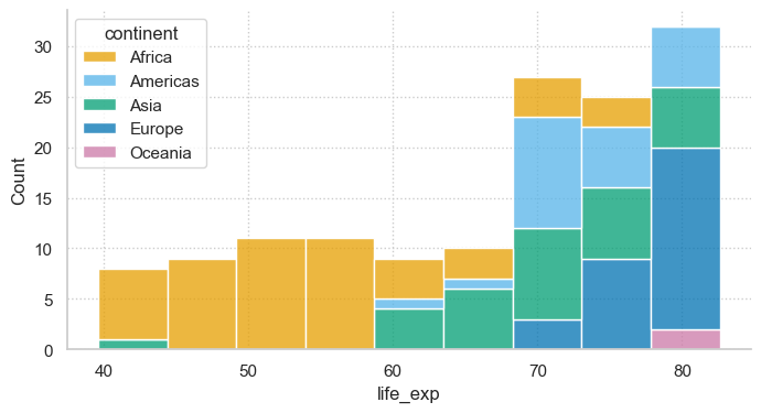
sns.set_theme(style="ticks", context="notebook", font_scale=1.05)
fig, ax = plt.subplots(figsize=(10, 6))
sns.scatterplot(data=gm07, x="gdp_per_cap", y="life_exp", hue="continent", size="pop_m", sizes=(30, 1200),
                palette=cont_colors, alpha=0.75, edgecolor="white", linewidth=0.8, ax=ax)
ax.set_xscale("log")
ax.xaxis.set_major_formatter(StrMethodFormatter("${x:,.0f}"))
for name in ["China", "India", "United States", "Japan", "Nigeria"]:
    r = gm07.loc[gm07["country"] == name].iloc[0]
    ax.annotate(name, (r["gdp_per_cap"], r["life_exp"]), xytext=(6, 6), textcoords="offset points", fontsize=9)
ax.set(xlabel="GDP per capita (USD, log scale)", ylabel="Life expectancy (years)")
ax.set_title("Richer countries live longer, but continent still matters (2007)", loc="left", fontweight="bold")
ax.text(0, -0.13, "Source: Gapminder. Bubble area proportional to population.", transform=ax.transAxes, fontsize=8, color="gray")
sns.move_legend(ax, "upper left", bbox_to_anchor=(1.01, 1), frameon=False, fontsize=9, labelspacing=1.4)
sns.despine()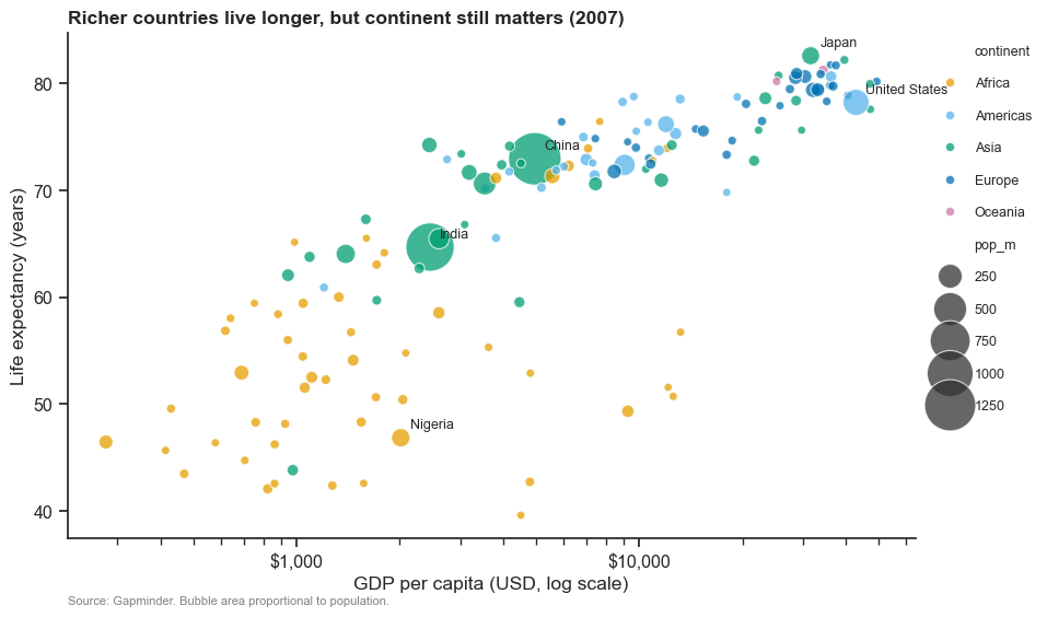
histplot, kdeplot, ecdfplot → facet with displotcountplot, barplot, boxplot, violinplot, stripplot → facet with catplotscatterplot, lineplot → facet with relplotregplot / lmplot, heatmap, jointplot, pairplothue, size, style, units; facets: col, row, col_wrapAxes; figure-level returns a grid with .figure and .axesset_theme(style, context, palette, font_scale, rc), axes_style, despine, move_legendhue="year")relplot of GDP per capita over time for 5 countries of your choice, one panel each, with a log y-axiscatplot of median life expectancy by continent with kind="bar", estimator="median", and your own palette dictionarycontext="poster", clean labels, annotation, and save it as a PDF