Explain the difference between a Figure and an Axes
Build any basic plot with one repeatable 5-step recipe
Pick the right plot type for your question (line, scatter, bar, histogram)
Customize colors, markers, labels, ticks, and legends
Arrange multiple plots in one figure with subplots
Save publication-quality figures
Turn a default plot into a professional one
How to use this notebook
Run the cells in order, top to bottom (Shift + Enter)
After each plot, change one number or keyword and re-run it: that is the fastest way to learn Matplotlib
The big picture
What is Matplotlib?
The foundational plotting library for Python, and still the most widely used
Created in 2003 by John D. Hunter, a neuroscientist who wanted MATLAB-quality plots in Python
Free, open source, and built on top of NumPy
Makes almost any 2D chart (and basic 3D), static or animated
Exports to PNG, PDF, SVG, and more, at publication quality
Bottom line: if a Python library draws a static chart, there is a good chance Matplotlib is doing the drawing
Where Matplotlib fits in the Python ecosystem
Think of it as a foundation layer that other tools build on:
Layer
Examples
What it gives you
High-level, built on Matplotlib
Seaborn, pandas .plot(), GeoPandas .plot()
Short commands for common statistical and DataFrame plots
Matplotlib
matplotlib.pyplot
Full control over every element of a figure
Numerical foundation
NumPy
The arrays of numbers being plotted
Separate interactive-web libraries (Plotly, Bokeh, Altair) use their own drawing engines and are aimed at browser dashboards.
Why learn Matplotlib first?
Seaborn and pandas plots return Matplotlib objects, so customizing them requires Matplotlib
Understanding the foundation makes every other plotting library easier
Analogy: Matplotlib is the paint and brushes; Seaborn is a paint-by-numbers kit built with them
Matplotlib vs. pyplot
matplotlib is the whole package: dozens of modules for colors, tick formatting, animation, 3D, file output, and more
matplotlib.pyplot is the one module you use day to day
A collection of MATLAB-style functions: plt.plot(), plt.subplots(), plt.savefig(), …
Keeps track of the “current” figure and plot for you behind the scenes
Your starting point for creating every figure
That is why every notebook begins with:
import matplotlib.pyplot as plt
You rarely import other parts of the package directly; pyplot and the objects it creates cover nearly everything in this course
How Matplotlib works under the hood
Three layers, from what you type to what you see:
Scripting layer (pyplot): the simple commands you write, e.g. plt.subplots()
Artist layer: everything visible on a plot is a Python object called an Artist
The Figure, each Axes, every line, tick, label, and legend
Customizing a plot = changing properties of these objects
Backend layer: turns the Artists into actual pixels or files
In Jupyter, an inline backend draws the figure under your cell
When saving, a file backend writes PNG, PDF, SVG, …
You almost never touch this layer directly
Takeaway: you write pyplot commands, they create and modify Artist objects, and the backend draws them.
Strengths and limitations
Strengths
Limitations
Total control over every detail
More code than higher-level libraries
Publication-quality static output
Default styling needs tuning to look professional
Works everywhere: notebooks, scripts, servers
Interactivity is limited compared to web libraries
Huge gallery of examples; mature and stable
Two coding styles (Section 3) confuse beginners
Use Matplotlib when you need a precise, polished figure for a report, paper, or slide deck, or when you need to fine-tune a plot made by Seaborn or pandas.
0. Setup
Install (only once, from the terminal, inside your conda environment):
Import (every notebook). These aliases are universal conventions, so always use them:
matplotlib.pyplot as plt: the plotting interface
numpy as np: fast arrays of numbers, used here to generate data
import matplotlibimport matplotlib.pyplot as pltimport numpy as npprint("Matplotlib version:", matplotlib.__version__)# Random number generator with a fixed seed, so everyone gets the same "random" datarng = np.random.default_rng(seed=42)
Matplotlib version: 3.10.8
Two NumPy functions you will see constantly in this notebook:
np.linspace(start, stop, n): n evenly spaced numbers from start to stop (great for smooth curves)
rng.normal(mean, std, n): n random numbers from a bell curve (great for fake “measured” data)
plt.plot(x, y) connected the points (1,1), (2,4), ..., (5,25) with straight lines
plt.show() rendered the figure
In Jupyter, the plot appears automatically at the end of a cell, so plt.show() is optional (but it hides extra text output, so it is a good habit)
In a regular .py script, plt.show() is required or nothing appears
Inputs can be Python lists, NumPy arrays, or pandas DataFrame columns; x and y just need the same length
2. Anatomy of a plot: Figure vs. Axes
Every Matplotlib plot is built from two main objects:
Figure: the whole canvas (the sheet of paper). Controls overall size, the overall title, and saving to file.
Axes: one individual plot inside the figure (one drawing on the paper). Holds the data, the axis labels, the title, the legend, the ticks.
A Figure can hold one or many Axes
Almost all plotting commands are methods of an Axes: ax.plot(), ax.set_xlabel(), ax.legend()
figure-vs-axes.png
Watch the spelling:
Axes = one whole plot panel (singular and plural are both “Axes”)
Axis = a single number line (the x-axis or the y-axis) inside an Axes
The labeled figure below names every component and the command that controls it. Keep it as a reference.
anatomy.png
3. Two ways to write Matplotlib code
You will see both styles online, so you need to recognize both.
Implicit (pyplot) style
Explicit (object-oriented) style
How it works
plt silently tracks the “current” figure and Axes
You create fig and ax and call methods on them
Looks like
plt.plot(), plt.xlabel()
ax.plot(), ax.set_xlabel()
Good for
Very quick, throwaway plots
Everything else, especially multiple plots
In this course we use the explicit style. It scales cleanly from one plot to many, and it is always clear which plot you are modifying.
x = [1, 2, 3, 4]y = [2, 4, 6, 8]# IMPLICIT STYLE: plt manages the figure and Axes behind the scenesplt.plot(x, y, marker="o")plt.title("Implicit style")plt.xlabel("Acceleration (m/s$^2$)")plt.ylabel("Force (N)")plt.show()
# EXPLICIT STYLE: we create the Figure and Axes ourselvesfig, ax = plt.subplots() # one Figure containing one Axesax.plot(x, y, marker="o")ax.set_title("Explicit style")ax.set_xlabel("Acceleration (m/s$^2$)")ax.set_ylabel("Force (N)")plt.show()
Same plot, slightly different names. Most Axes methods just add set_:
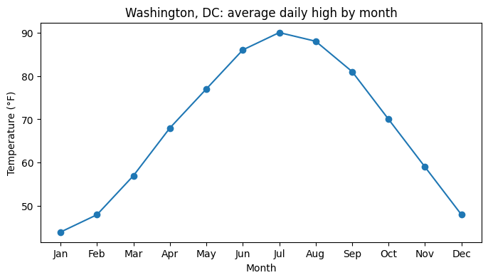
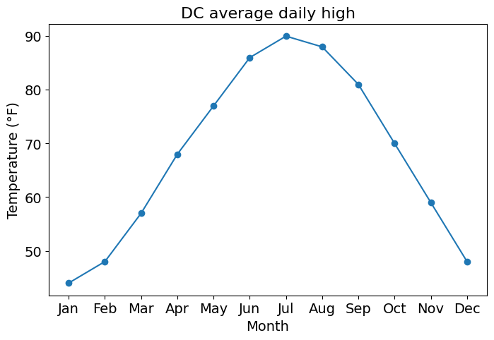
# 1. DATA: approximate average daily high temperature in Washington, DCmonths = ["Jan", "Feb", "Mar", "Apr", "May", "Jun","Jul", "Aug", "Sep", "Oct", "Nov", "Dec"]dc_high = [44, 48, 57, 68, 77, 86, 90, 88, 81, 70, 59, 48]# 2. CREATEfig, ax = plt.subplots(figsize=(8, 4))# 3. PLOTax.plot(months, dc_high, marker="o")# 4. LABELax.set_title("Washington, DC: average daily high by month")ax.set_xlabel("Month")ax.set_ylabel("Temperature (°F)")# 5. SAVE / SHOW# fig.savefig("dc_temps.png", dpi=300, bbox_inches="tight") # (covered in Section 11)plt.show()
Notice that x can be text (the month names). Matplotlib treats them as ordered categories.
5. Subplots: many Axes in one Figure
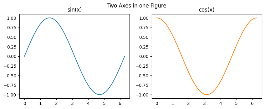
plt.subplots(nrows, ncols) creates a grid of Axes.
With one plot, ax is a single Axes object
With several plots, you get back a NumPy array of Axes, so you pick one with indexing:
One row or one column: axs[0], axs[1], …
A 2D grid: axs[row, col], e.g. axs[0, 1] is top row, second column
x = np.linspace(0, 2* np.pi, 200)fig, axs = plt.subplots(1, 2, figsize=(10, 3.5)) # 1 row, 2 columnsprint(type(axs), axs.shape)axs[0].plot(x, np.sin(x))axs[0].set_title("sin(x)")axs[1].plot(x, np.cos(x), color="tab:orange")axs[1].set_title("cos(x)")fig.suptitle("Two Axes in one Figure") # title for the whole Figureplt.show()
<class 'numpy.ndarray'> (2,)
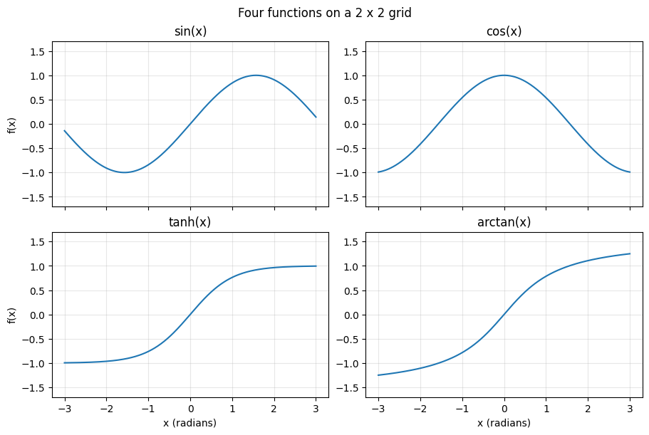
Three settings that make subplots look right:
layout="constrained": automatically spaces plots so labels never overlap (use it every time)
sharex=True / sharey=True: subplots use the same axis range, which makes them directly comparable
for ax in axs.flat: loops over every Axes in a grid, so you can apply the same settings to all of them
funcs = [np.sin, np.cos, np.tanh, np.arctan]names = ["sin(x)", "cos(x)", "tanh(x)", "arctan(x)"]x = np.linspace(-3, 3, 400)fig, axs = plt.subplots(2, 2, figsize=(9, 6), sharex=True, layout="constrained")for ax, f, name inzip(axs.flat, funcs, names): ax.plot(x, f(x)) ax.set_title(name) ax.set_ylim(-1.7, 1.7) ax.grid(alpha=0.3)# Label only the outer edges of the gridfor ax in axs[1, :]: ax.set_xlabel("x (radians)")for ax in axs[:, 0]: ax.set_ylabel("f(x)")fig.suptitle("Four functions on a 2 x 2 grid")plt.show()
6. Choosing the right plot type
Start from the question, not the chart. Then pick the plot that answers it.
Your question
Plot type
Axes method
How does something change over time or an ordered variable?
Line
ax.plot()
How are two numeric variables related?
Scatter
ax.scatter()
How do categories compare?
Bar
ax.bar() / ax.barh()
How is one numeric variable distributed?
Histogram
ax.hist()
6.1 Line plot: change over an ordered x
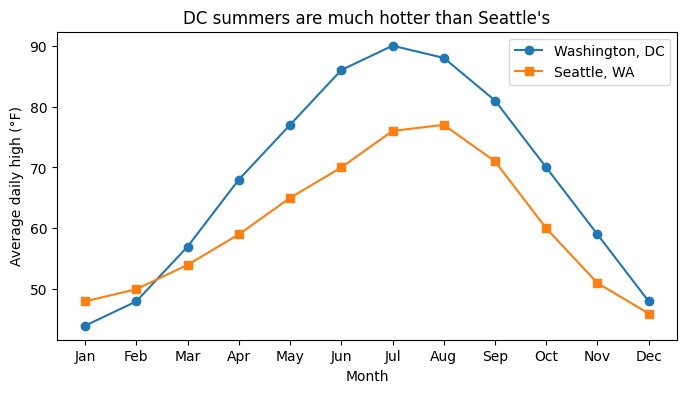
Call ax.plot() once per line; each call adds to the same Axes
Give each line a label= and call ax.legend() to identify them
# Approximate average daily highs (°F)seattle_high = [48, 50, 54, 59, 65, 70, 76, 77, 71, 60, 51, 46]fig, ax = plt.subplots(figsize=(8, 4))ax.plot(months, dc_high, marker="o", label="Washington, DC")ax.plot(months, seattle_high, marker="s", label="Seattle, WA")ax.set_title("DC summers are much hotter than Seattle's")ax.set_xlabel("Month")ax.set_ylabel("Average daily high (°F)")ax.legend()plt.show()
6.2 Scatter plot: relationship between two variables
Each point is one observation; no lines connect them
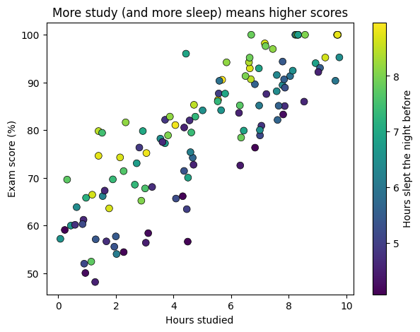
Encode a third variable with color (c=) and add a colorbar to explain it
n =120hours_studied = rng.uniform(0, 10, n)hours_slept = rng.uniform(4, 9, n)exam_score = np.clip(40+4* hours_studied +3* hours_slept + rng.normal(0, 6, n), 0, 100)fig, ax = plt.subplots(figsize=(7, 5))points = ax.scatter(hours_studied, exam_score, c=hours_slept, cmap="viridis", s=50, edgecolor="black", linewidth=0.5)fig.colorbar(points, ax=ax, label="Hours slept the night before")ax.set_title("More study (and more sleep) means higher scores")ax.set_xlabel("Hours studied")ax.set_ylabel("Exam score (%)")plt.show()
6.3 Bar chart: compare categories
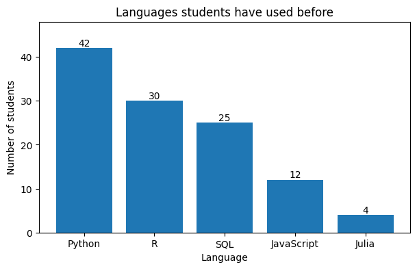
ax.bar(categories, values) for vertical bars
ax.barh() for horizontal bars: better when category names are long or there are many categories
Order the bars (largest to smallest) so the ranking is obvious at a glance
ax.bar_label() writes the value on each bar
languages = ["Python", "R", "SQL", "JavaScript", "Julia"]n_students = [42, 30, 25, 12, 4] # illustrative survey countsfig, ax = plt.subplots(figsize=(7, 4))bars = ax.bar(languages, n_students, color="tab:blue")ax.bar_label(bars)ax.set_ylim(0, 48) # headroom so the top label fitsax.set_title("Languages students have used before")ax.set_xlabel("Language")ax.set_ylabel("Number of students")plt.show()
6.4 Histogram: distribution of one variable
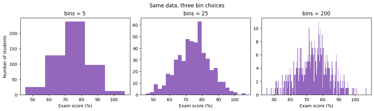
Splits the values into bins and counts how many fall in each
The number of bins changes the story: too few hides detail, too many looks noisy
9. Controlling the axes: limits, ticks, scales, grid
Command
Purpose
ax.set_xlim(lo, hi) / ax.set_ylim(lo, hi)
Zoom to a range
ax.set_xticks([...])
Choose where ticks go
ax.set_xticks([...], ["a", "b", ...])
Choose ticks and their text labels
ax.tick_params(labelsize=14, rotation=45)
Tick label size / rotation
ax.set_yscale("log")
Logarithmic axis
ax.grid(True, alpha=0.3)
Light background grid
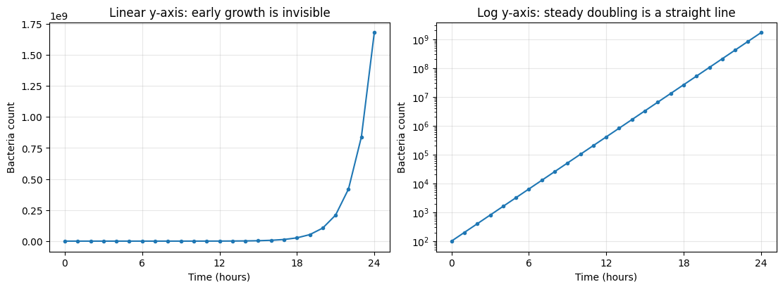
When to use a log scale: data that spans several orders of magnitude, or grows exponentially. On a log axis, exponential growth becomes a straight line.
hours = np.arange(0, 25)bacteria =100*2** hours # population doubles every hourfig, axs = plt.subplots(1, 2, figsize=(11, 4), layout="constrained")axs[0].plot(hours, bacteria, marker=".")axs[0].set_title("Linear y-axis: early growth is invisible")axs[1].plot(hours, bacteria, marker=".")axs[1].set_yscale("log")axs[1].set_title("Log y-axis: steady doubling is a straight line")for ax in axs: ax.set_xlabel("Time (hours)") ax.set_ylabel("Bacteria count") ax.set_xticks([0, 6, 12, 18, 24]) ax.grid(True, alpha=0.3)plt.show()
10. Changing the defaults: rcParams
Instead of passing fontsize= to every single command, change Matplotlib’s defaults.
Defaults live in plt.rcParams, which works like a Python dictionary
Permanent (for the rest of the notebook): plt.rcParams.update({...})
Temporary (one plot only): with plt.rc_context({...}):
Style sheets (pre-made looks, e.g. "ggplot"): plt.style.use("ggplot"); list them with plt.style.available
print("Default figure size (inches):", plt.rcParams["figure.figsize"])print("Default font size: ", plt.rcParams["font.size"])
Default figure size (inches): [6.4, 4.8]
Default font size:            10.0
# PERMANENT: bigger, more readable defaults for every plot from here onplt.rcParams.update({"font.size": 14,"axes.titlesize": 16,"axes.labelsize": 14,"legend.fontsize": 12,"figure.figsize": (8, 5),})# To undo all changes and restore Matplotlib's factory defaults:# plt.rcdefaults()
Tip: put a plt.rcParams.update({...}) cell at the top of every notebook you write. Every plot instantly looks more consistent and readable.
.png: images for slides, websites, reports (raster; set dpi=300 for sharp results)
.pdf / .svg: vector graphics that stay sharp at any zoom (best for papers and LaTeX)
bbox_inches="tight": trims extra white space and prevents labels from being cut off
Save before plt.show(): in scripts, show() can clear the figure, giving you a blank file
fig, ax = plt.subplots()ax.plot(months, dc_high, marker="o")ax.set(title="DC average daily high", xlabel="Month", ylabel="Temperature (°F)")fig.savefig("dc_temps.png", dpi=300, bbox_inches="tight") # 1. savefig.savefig("dc_temps.pdf", bbox_inches="tight")plt.show() # 2. then showprint("Saved dc_temps.png and dc_temps.pdf to the current folder")
Saved dc_temps.png and dc_temps.pdf to the current folder
12. From default to professional
Guidelines for good visualizations
These are the minimum standard for every plot you submit in the DSAN program. Plots that ignore them consistently lose points.
Descriptive labels with units
"price" is bad: price of what? in what currency?
"S&P 500 index price (US dollars)" is good
Large fonts
Plots end up in slides and must be readable from the back of the room
Roughly 14 to 20 pt for labels and ticks; not comically large
Don’t overplot
One or two messages per plot; split the rest into subplots or separate figures
Always have a message
No “plots for plots’ sake”; a good title often states the takeaway
No overlapping text
Use layout="constrained", rotate tick labels, or move the legend
Before and after
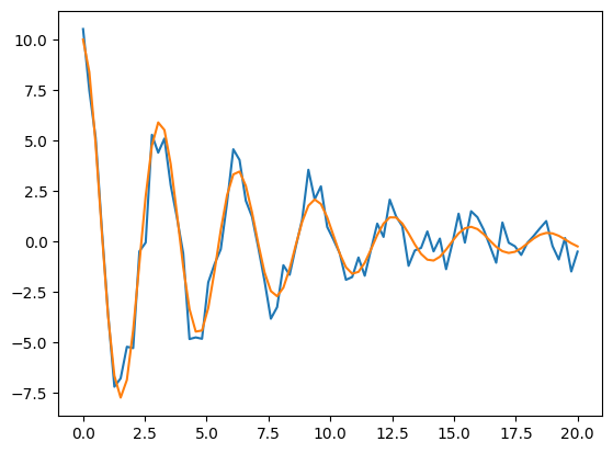
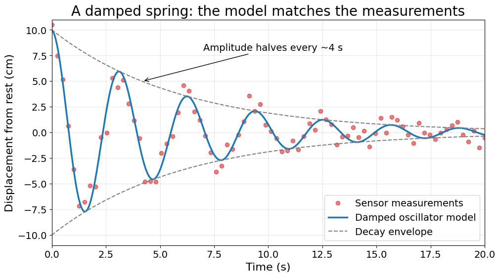
Same data both times: noisy measurements of a spring that slowly stops bouncing.
t = np.linspace(0, 20, 80) # time (s)model =10* np.exp(-t /6) * np.cos(2* t) # true motion (cm)measured = model + rng.normal(0, 0.8, t.size) # noisy sensor readings# BEFORE: pure defaultsplt.rcdefaults() # temporarily go back to factory defaults for a fair comparisonfig, ax = plt.subplots()ax.plot(t, measured)ax.plot(t, model)plt.show()
What’s wrong: no title, no labels, no units, no legend, tiny fonts, and it is unclear which line is data and which is the model.
Checklist that the “after” plot satisfies: clear takeaway in the title, units on both axes, readable fonts, data and model visually distinct (markers vs. line), legend, light grid, one annotation that supports the message, nothing overlapping.
13. Common errors and how to fix them
Symptom / error message
Cause
Fix
AttributeError: 'Axes' object has no attribute 'xlabel'
Mixed up pyplot and Axes names
Use ax.set_xlabel() (see table in Section 3)
AttributeError: 'numpy.ndarray' object has no attribute 'plot'
With subplots, axs is an array of Axes
Index it: axs[0].plot() or axs[0, 1].plot()
ValueError: x and y must have same first dimension