import networkx as nx
import matplotlib.pyplot as plt

#GENERATE GRAPH
# G = nx.complete_graph(20)
G= nx.erdos_renyi_graph(30,0.4)

#BASIC PLOT (defaults)
pos=nx.random_layout(G)
nx.draw(G,pos=pos)
plt.show()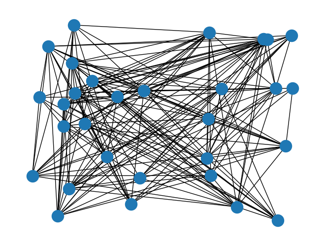
Typically we plot networks in 2D, but to do so we need x,y positions for each node
In short: Canonical = “accepted” or “standard”
Generally, graph visualization methods fall into two main categories:
Geometric Layouts
Use explicit rules or graph-theoretic metrics (e.g., node degree, hierarchy, coordinates)
Examples:
Force-Directed Layouts
Recall that degree centrality is the number of edges connected to a node.
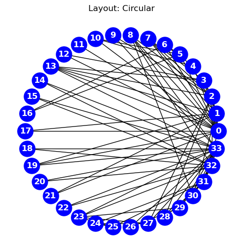
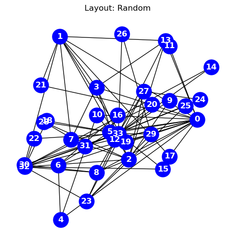
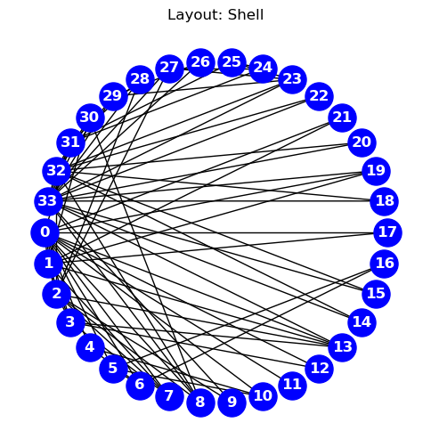
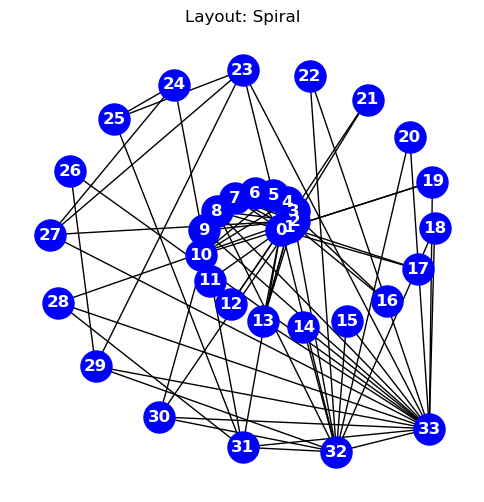
Geometric layouts assign node positions based on geometric rules or graph properties, not optimization.
The primary benefit of these methods is that they are simple, fast, deterministic, and reproducible.
Nodes \(i = 1, \dots, N\) placed evenly on a circle:
\[ x_i = R \cos\left(\frac{2\pi i}{N}\right), \quad y_i = R \sin\left(\frac{2\pi i}{N}\right) \]
where \(R\) is the radius, and \(i\) is the node index.
Nodes placed in a regular 2D grid:
\[ x_i = i \bmod C, \quad y_i = \left\lfloor \frac{i}{C} \right\rfloor \]
where \(C\) is the number of columns in the grid.
import networkx as nx
import matplotlib.pyplot as plt
#GENERATE GRAPH
# G = nx.complete_graph(20)
G= nx.erdos_renyi_graph(30,0.4)
#BASIC PLOT (defaults)
pos=nx.random_layout(G)
nx.draw(G,pos=pos)
plt.show()
import networkx as nx
import matplotlib.pyplot as plt

#CUSTOMIZE
#specifiy x-y positions for plotting
pos=nx.circular_layout(G)

#initialize plot
fig, ax = plt.subplots()
nx.draw(
G,
node_color='blue',
edgecolors="black",
edge_color="black",
linewidths=2,
font_color="white",
font_weight="bold",
node_size=500,
width=2,
with_labels=True,
pos=pos,
ax=ax
)
ax.set(title='Basic NetworkX plot')
ax.set_aspect('equal', 'box')
#fig.savefig("test.png")
plt.show()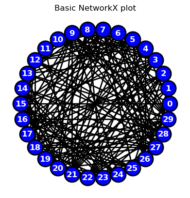
Nodes are arranged by depth and breadth in a tree or DAG:
\[ y_i = -\text{depth}(i), \quad x_i = \text{assigned based on order within level} \]
Often uses DFS/BFS traversal to assign horizontal spacing.
Uses the second and third smallest eigenvectors of the graph Laplacian \(L\):
\[ (x_i, y_i) = (\mathbf{v}_2[i], \mathbf{v}_3[i]) \]
where \(\mathbf{v}_2\), \(\mathbf{v}_3\) are the Fiedler vectors, giving a low-dimensional embedding.
Positions are externally defined:
\[ (x_i, y_i) = (\text{longitude}_i, \text{latitude}_i) \]
| Feature | Geometric Layouts | Force-Directed Layouts |
|---|---|---|
| Basis | Deterministic rules | Physical simulation |
| Node Positioning | Fixed rules (e.g. grid) | Emerges from graph structure |
| Flexibility | Low | High |
| Community Detection | Poor | Strong |
| Real-world Interpretability | Good (for spatial graphs) | Good (for topology insight) |
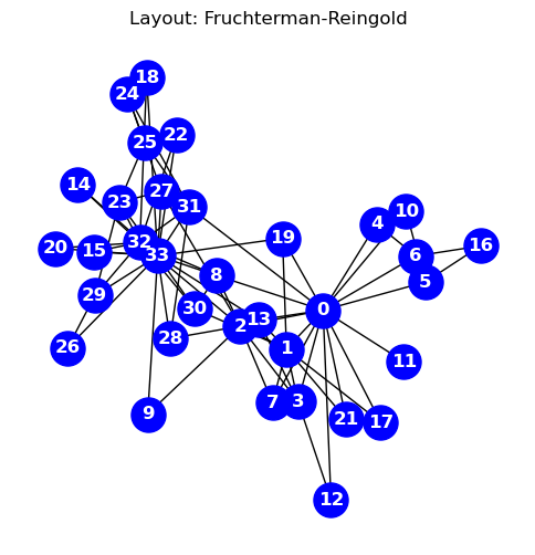
Fruchterman-Reingold treats nodes like repelling magnets and edges like springs drawing connected nodes together. It balances these forces to cluster related nodes and separate unrelated ones, iteratively adjusting positions for a clear structure.
For example: - A singleton node (no connections) drifts to the side, away from clusters. - A node with one connection stays near its neighbor, usually at the edge. - A hub node (many connections) is pulled from all sides, settling near the center to reflect its importance.
This layout naturally reveals clusters, central nodes, and the graph’s main structure.
Inputs:
Variables:
Objective Function: \(E\): Total system energy
\[ E = \sum_{i \ne j} f_r(d_{ij}) + \sum_{(i,j) \in E} f_a(d_{ij}) \]
Where:
\(d_{ij} = \| (x_i, y_i) - (x_j, y_j) \|\)
Repulsive force between all pairs:
\[ f_r(d) = -\frac{k^2}{d} \]
Attractive force along edges:
\[ f_a(d) = \frac{d^2}{k} \]
\(k \sim \sqrt{\frac{\text{area}}{N}}\): optimal pairwise distance
Note on the physics of the potential function:
Optimization Procedure:
Output: 2D coordinates \(\{(x_i, y_i)\}\) minimizing energy
#CUSTOMIZE
#specifiy x-y positions for plotting
pos=nx.spring_layout(G,iterations=200)

#initialize plot
fig, ax = plt.subplots()
nx.draw(
G,
node_color='blue',
edgecolors="black",
edge_color="black",
linewidths=2,
font_color="white",
font_weight="bold",
node_size=500,
width=2,
with_labels=True,
pos=pos,
ax=ax
)
ax.set(title='Basic NetworkX plot')
ax.set_aspect('equal', 'box')
#fig.savefig("test.png")
plt.show()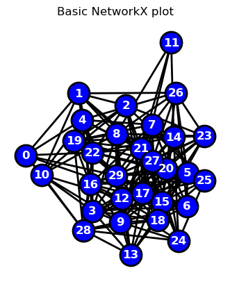
Inputs:
Variables:
Objective Function`: \(( E )\): Spring energy
\[ E = \frac{1}{2} \sum_{i < j} K_{ij} \left( \| (x_i, y_i) - (x_j, y_j) \| - L_{ij} \right)^2 \]
Where:
Optimization Procedure:
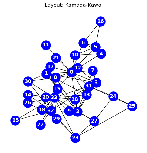
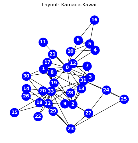
Output: 2D coordinates \(\{(x_i, y_i)\}\) approximating graph-theoretic distances
| Feature | Fruchterman-Reingold | Kamada-Kawai |
|---|---|---|
| Goal | Balance attractive and repulsive forces for visual clarity | Make Euclidean distances reflect shortest-path distances in the graph |
| Forces Used | Repulsion between all node pairs; attraction along edges | Spring-like forces between all node pairs based on graph distances |
| Input Requirements | Graph structure (adjacency list or matrix) | Graph structure + all-pairs shortest path distances |
| Energy Function | Heuristic energy with separate attractive and repulsive terms | Total spring energy: deviation from ideal pairwise distances |
| Force Formulation | - Repulsion: \(f_r(d) = -\frac{k^2}{d}\) (between all pairs) - Attraction: \(f_a(d) = \frac{d^2}{k}\) (along edges) |
- Spring force: \(f_{ij} = k_{ij} \left( d_{ij}^{\text{actual}} - L_{ij} \right) \frac{\vec{x}_i - \vec{x}_j}{d_{ij}^{\text{actual}}}\) |
| Optimization Approach | Iterative position updates via simulated annealing or cooling | Gradient-based optimization using Newton-Raphson method |
| Computational Cost | \(O(n^2)\) (with approximations like Barnes-Hut for scalability) | \(O(n^2)\) (due to full pairwise shortest-path and forces) |
| Strengths | Fast, intuitive clusters, adaptable to sparse or large graphs | Preserves global structure and relative distances with high fidelity |
| Weaknesses | May distort long-range structure; lacks true distance meaning | Computationally intensive; doesn’t scale well to large graphs |
| Supports Edge Weights | Optional; scales attractive forces | Yes; directly used to compute ideal lengths \(L_{ij}\) |
| Output | 2D coordinates revealing structure via force balance | 2D coordinates approximating graph-theoretic distances |
import networkx as nx
import matplotlib.pyplot as plt

#GENERATE A COMPLETE GRAPH USING A GRAPH GENERATOR
#https://networkx.org/documentation/stable/reference/generators.html
# G = nx.complete_graph(10)
# G = nx.gnp_random_graph(25,p=0.7)
# G=nx.barabasi_albert_graph(30,2)
G=nx.karate_club_graph()

for i in range(0,3+1):
    #print(i)
    #CAN MANUALLY SPECIFY GRAPH LOCATIONS WITH A DICTIONARY OF (X,Y) ARRAYS
    if(i==1):
        title="Layout: Manual"; pos={}; j=0; i1=0
        for k in range(0,len(list(G.edges))):
            if(k%5==0): j=j+1
            if(k%5==0): i1=0
            i1=i1+1
            pos[k]=[j,i1]

    # OR YOU CAN USE ONE OF NETWORK-X'S BUILT-IN POSITION LAYOUT ALGORITHMS
    if(i==0): title="Layout: Random";     pos = nx.random_layout(G)
    if(i==1): title="Layout: Fruchterman-Reingold";     pos = nx.spring_layout(G)
    if(i==2): title="Layout: Kamada-Kawai";     pos = nx.kamada_kawai_layout(G)

    fig, ax = plt.subplots()
    fig.set_size_inches(6, 6)

    nx.draw(
        G,
        node_color="blue",
        node_size=500,
        font_color="white",
        font_weight="bold",
        with_labels=True,
        pos=pos,
    )
    ax.set(title=title)
    # if(i>1): ax.set_aspect('equal', 'box')
    plt.title(title)
    plt.show()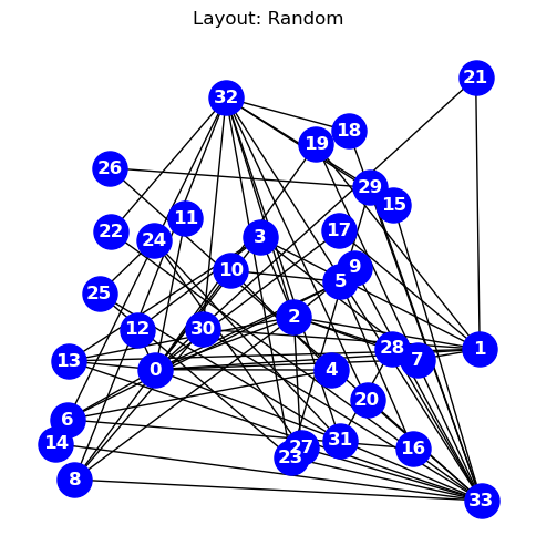
Here are the geometric layout functions provided by NetworkX (as of recent versions):
circular_layout(G)
shell_layout(G)
spring_layout(G) (force-directed, but often grouped with geometric)
kamada_kawai_layout(G)
spectral_layout(G)
random_layout(G)
spiral_layout(G)
rescale_layout(pos) (utility function)
import networkx as nx
import matplotlib.pyplot as plt

#GENERATE A COMPLETE GRAPH USING A GRAPH GENERATOR
#https://networkx.org/documentation/stable/reference/generators.html
# G = nx.complete_graph(10)
# G = nx.gnp_random_graph(25,p=0.7)
# G=nx.barabasi_albert_graph(30,2)
G=nx.karate_club_graph()

for i in range(1,5+1):
    #print(i)
    #CAN MANUALLY SPECIFY GRAPH LOCATIONS WITH A DICTIONARY OF (X,Y) ARRAYS
    if(i==1):
        title="Layout: Manual"; pos={}; j=0; i1=0
        for k in range(0,len(list(G.edges))):
            if(k%5==0): j=j+1
            if(k%5==0): i1=0
            i1=i1+1
            pos[k]=[j,i1]

    # OR YOU CAN USE ONE OF NETWORK-X'S BUILT-IN POSITION LAYOUT ALGORITHMS
    if(i==1): title="Layout: Spectral";     pos = nx.spectral_layout(G)
    if(i==2): title="Layout: Circular";     pos = nx.circular_layout(G)
    if(i==3): title="Layout: Random";       pos = nx.random_layout(G)
    if(i==4): title="Layout: Shell";        pos = nx.shell_layout(G)
    if(i==5): title="Layout: Spiral";        pos = nx.spiral_layout(G)


    fig, ax = plt.subplots()
    fig.set_size_inches(6, 6)

    nx.draw(
        G,
        node_color="blue",
        node_size=500,
        font_color="white",
        font_weight="bold",
        with_labels=True,
        pos=pos,
    )
    ax.set(title=title)
    # if(i>1): ax.set_aspect('equal', 'box')
    plt.title(title)
    plt.show()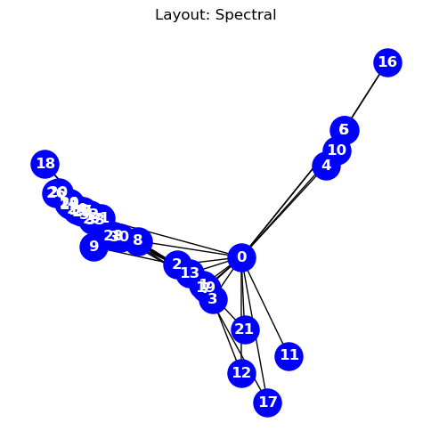
In the following self-contained example we show how to add various customization options to a NetworkX plot
import networkx as nx
import matplotlib.pyplot as plt
import random
import numpy as np

#GENERATE GRAPH
N=20

G = nx.complete_graph(N)
G = nx.gnp_random_graph(N, 0.1, seed=10374196)

#ASSIGN RANDOM ATTRIBUTES TO NODES+EDGES
for u in G.nodes(): G.nodes[u]['attribute']=0.2+1*random.uniform(0, 1)
for u,v in G.edges(): G[u][v]['weight']=5*random.uniform(0, 1)

#PRINT NODE+EDGES
for node in G.nodes(data=True): print(node)
for line in nx.generate_edgelist(G, data=True): print(line)

#SPECIFIY X-Y POSITIONS FOR PLOTTING
# pos=nx.circular_layout(G)
pos=nx.spring_layout(G,k=50*1./np.sqrt(N),iterations=500)
# pos=nx.random_layout(G)

#GENERATE PLOT
fig, ax = plt.subplots()
fig.set_size_inches(10, 10)

#assign colors based on attributes
weights_n   = [G.nodes[u]['attribute'] for u in G.nodes()]
weights_e   = [G[u][v]['weight'] for u,v in G.edges()]

#SAMPLE CMAP FOR COLORS
cmap=plt.cm.get_cmap('Blues')
colors_e    = [cmap(G[u][v]['weight']/5.0) for u,v in G.edges()]
colors_n    = [cmap(G.nodes[u]['attribute']/1.2) for u in G.nodes()]

#VARIOUS METHODS FOR VISUALIZING SIZE

#LABELS (DICT)
labels={}
for n,d in nx.degree(G): labels[n]=d #str(n)+"-"+str(d)

#WEIGHTS
# node_size=1000*weights_n

#DEGREE CENTRALITY
centrality=nx.degree(G)
centrality=np.array([d for n,d in centrality]); #print(G_DEGREE)
node_size=1000*centrality/max(centrality)
colors_n = node_size
colors_n = [cmap(u/max(centrality)) for u in centrality]

#PLOT
nx.draw(
G,
    node_color=colors_n,
    edgecolors="black",
    edge_color=colors_e,
    linewidths=2,
    labels=labels,
    font_color="white",
    font_weight="bold",
    node_size=node_size,
    width=weights_e,
    with_labels=True,
    pos=pos,
    ax=ax
)

#TITLE
ax.set(title='Color and size plotted by attribute')
ax.set_aspect('equal', 'box')

#PLOT
# fig.savefig("test.png")
plt.show()
(0, {'attribute': 0.3919447950819344})
(1, {'attribute': 0.5478313825613723})
(2, {'attribute': 0.4813642741523469})
(3, {'attribute': 0.6442768796202429})
(4, {'attribute': 0.5492450916307241})
(5, {'attribute': 0.4920965363771432})
(6, {'attribute': 1.1553568196555102})
(7, {'attribute': 0.9200500943715493})
(8, {'attribute': 0.964457258484575})
(9, {'attribute': 1.1650523088335885})
(10, {'attribute': 0.5433476199336214})
(11, {'attribute': 0.8773580860481529})
(12, {'attribute': 0.2919521524284893})
(13, {'attribute': 0.39015823441290737})
(14, {'attribute': 0.9344950626927089})
(15, {'attribute': 0.3060254057351261})
(16, {'attribute': 0.8358897211018044})
(17, {'attribute': 0.7806892197266564})
(18, {'attribute': 1.176516867772237})
(19, {'attribute': 0.9486454327580556})
0 14 {'weight': 2.0233618168520415}
1 14 {'weight': 3.2459758416891713}
2 9 {'weight': 2.433604791548147}
2 11 {'weight': 2.153010085713147}
3 9 {'weight': 4.236227463860567}
3 12 {'weight': 3.091841566151514}
4 11 {'weight': 0.4524424256557763}
4 12 {'weight': 0.701795302799893}
4 15 {'weight': 3.7497482817772876}
5 12 {'weight': 0.44579261489398725}
5 13 {'weight': 4.009348009739661}
5 15 {'weight': 2.830109958683687}
5 17 {'weight': 2.0024789396952953}
6 19 {'weight': 2.0838525261138057}
7 14 {'weight': 2.8409080419790538}
7 18 {'weight': 0.027748399519490485}
8 9 {'weight': 4.232640584915755}
8 17 {'weight': 4.872296914164571}
10 13 {'weight': 2.166287275637596}
10 17 {'weight': 0.833852622800515}
10 18 {'weight': 4.116621684344794}
11 13 {'weight': 1.7171225557676317}
12 19 {'weight': 2.35869079393336}
13 15 {'weight': 0.4458025401201965}
13 18 {'weight': 1.5026317294248337}
14 15 {'weight': 0.650428348589075}/var/folders/lc/n91cn5z96ws6f52d25t2rpbh0000gn/T/ipykernel_6917/2235291110.py:34: MatplotlibDeprecationWarning: The get_cmap function was deprecated in Matplotlib 3.7 and will be removed in 3.11. Use ``matplotlib.colormaps[name]`` or ``matplotlib.colormaps.get_cmap()`` or ``pyplot.get_cmap()`` instead.
cmap=plt.cm.get_cmap('Blues')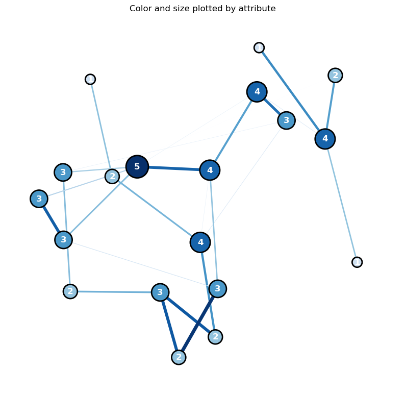
# MODIFIED FROM
# https://networkx.org/documentation/stable/auto_examples/drawing/plot_degree.html
import networkx as nx
import numpy as np
import matplotlib.pyplot as plt

#-------------------
# PLOTTING FUNCTION
#-------------------
def degree_histogram_plot(G):
    #COMPUTE DEGREE: --> "LIST" WITH NODE DEGREES
    G_DEGREE=G.degree(); #print(G_DEGREE,G_DEGREE[5],type(G_DEGREE))

    #LABELS (DICT)
    labels={}
    for n,d in G_DEGREE: labels[n]=d #str(n)+"-"+str(d)

    #SORT DEGREE AND STORE IN LIST
    degree_sequence = sorted((d for n, d in G_DEGREE), reverse=True)
    dmax = max(degree_sequence)   #MAX DEGREE

    #INITIALIZE MPL FIGURE+AX
    fig = plt.figure("Degree of a random graph", figsize=(10, 10))
    # Create a gridspec for adding subplots of different sizes
    axgrid = fig.add_gridspec(5, 4)

    #PLOT NETWORK IN UPPER GRID SPACES
    ax0 = fig.add_subplot(axgrid[0:3, :])
    pos = nx.spring_layout(G)
    nx.draw(G,
        with_labels=True,
        labels=labels,
        node_color='blue',
        node_size=500,
        font_color='white',
        font_size=16,
        pos=pos,ax=ax0
        )
    ax0.set_title("Network Graph: G")

    #PLOT RANK (IMPORTANCE BASED ON DEGREE) VS DEGREE)
    ax1 = fig.add_subplot(axgrid[3:, :2])
    ax1.plot(degree_sequence, "b-", marker="o")
    ax1.set_title("Degree Rank Plot")
    ax1.set_ylabel("Degree")
    ax1.set_xlabel("Rank")

    #PLOT RANK HISTOGRAM
    ax2 = fig.add_subplot(axgrid[3:, 2:])
    ax2.bar(*np.unique(degree_sequence, return_counts=True))
    ax2.set_title("Degree histogram")
    ax2.set_xlabel("Degree")
    ax2.set_ylabel("# of Nodes")
    ax0.set_aspect('equal', 'box')
    fig.tight_layout()
    plt.show()

    print(
    "NETWORK DENSITY:", nx.density(G), "\n",
    "NETWORK DIAMETER:", nx.diameter(G), "\n",
    )

#-------------------
#GENERATE GRAPHS+PLOT
#-------------------
print("RANDOM GRAPH")
#gnp_random_graph(n, p=, seed=None, directed=False)
#p=connection probablity
G = nx.gnp_random_graph(100, 0.2, seed=10374196)
degree_histogram_plot(G)

print("COMPLETE GRAPH")
G = nx.complete_graph(50)
degree_histogram_plot(G)

print("BINOMIAL TREE")
G = nx.binomial_tree(7)
degree_histogram_plot(G)
RANDOM GRAPH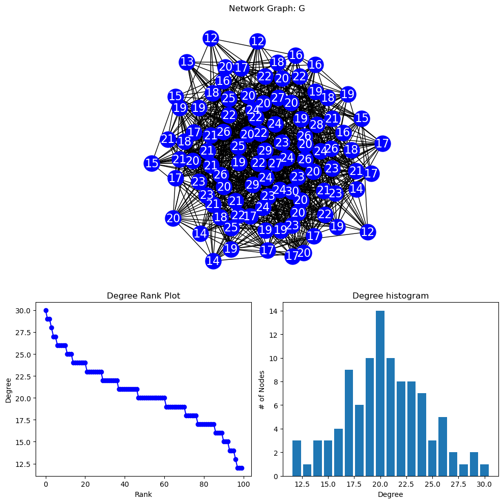
NETWORK DENSITY: 0.20646464646464646
 NETWORK DIAMETER: 3

COMPLETE GRAPH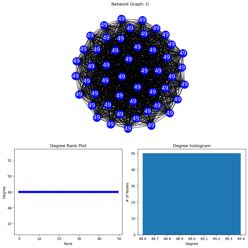
NETWORK DENSITY: 1.0
 NETWORK DIAMETER: 1

BINOMIAL TREE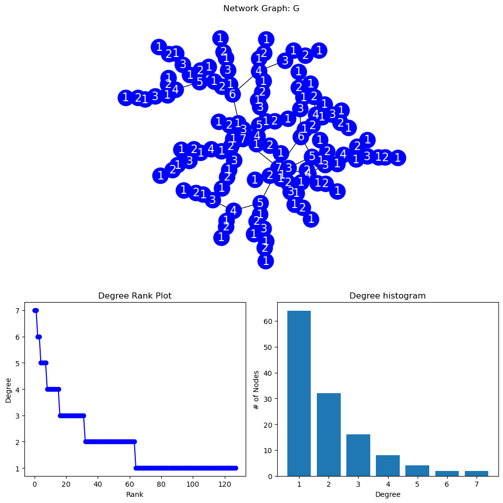
NETWORK DENSITY: 0.015625
 NETWORK DIAMETER: 13