---
title: "R Fundamentals"
format:
  html: default
  ipynb: default
---Review Fundamentals
A working refresher on the R language, followed by a first look at the tidyverse
- Part 2: data structures
- Part 3: control flow and functions
- Part 4: the tidyverse
Run every cell as we go. The fastest way to learn R is to break things and read the error.
Aside: Data driven narrative
https://www.reuters.com/graphics/GLOBAL-ENVIRONMENT/INSECT-APOCALYPSE/egpbykdxjvq/
Formatting
The following cell tells IRkernel not to generate text/latex output, don’t worry about the details associated with this cell
# Tells IRkernel not to generate text/latex output
options(jupyter.display_mimetypes = c(
  "text/plain",
  "text/html",
  "text/markdown",
  "image/svg+xml",
  "image/png",
  "image/jpeg"
))
Part 1: The Basics
Why R
- Built by statisticians, for data: modeling, inference, and graphics are first-class
- Vectors are the native unit of computation, not single values
- Huge package ecosystem on CRAN, with strong tooling for reproducible reports
- Two dialects coexist: base R (this notebook, Part 1 to 3) and the tidyverse (Part 4 and 5)
Assignment and printing
<-is the conventional assignment operator;=also works but is reserved by habit for function arguments#starts a comment- A bare object name prints itself;
print()andcat()do it explicitly
x <- 5          # preferred
y = 3           # legal, less idiomatic
z <- x + y

z               # auto-print
print(z)        # explicit print
cat("z is", z, "\n")   # cat: no quotes, no index marker
8
[1] 8
z is 8
Arithmetic operators
+ - * / ^behave as expected%%is modulo (remainder),%/%is integer division- R follows standard operator precedence; parentheses win
7 + 2
7 / 2
7 %% 2      # remainder
7 %/% 2     # integer division
2^10
sqrt(16)
round(3.14159, 2)
9
3.5
1
3
1024
4
3.14
Comparison and logical operators
- Comparison:
== != < > <= >= - Logical:
&(and),|(or),!(not) - Comparisons return
TRUEorFALSE, which are themselves a data type
5 > 3
5 == 5
5 != 5

(5 > 3) & (2 > 1)     # both must be TRUE
(5 > 3) | (2 > 10)    # at least one TRUE
!(5 > 3)              # negation
TRUE
TRUE
FALSE
TRUE
TRUE
FALSE
The fundamental data types
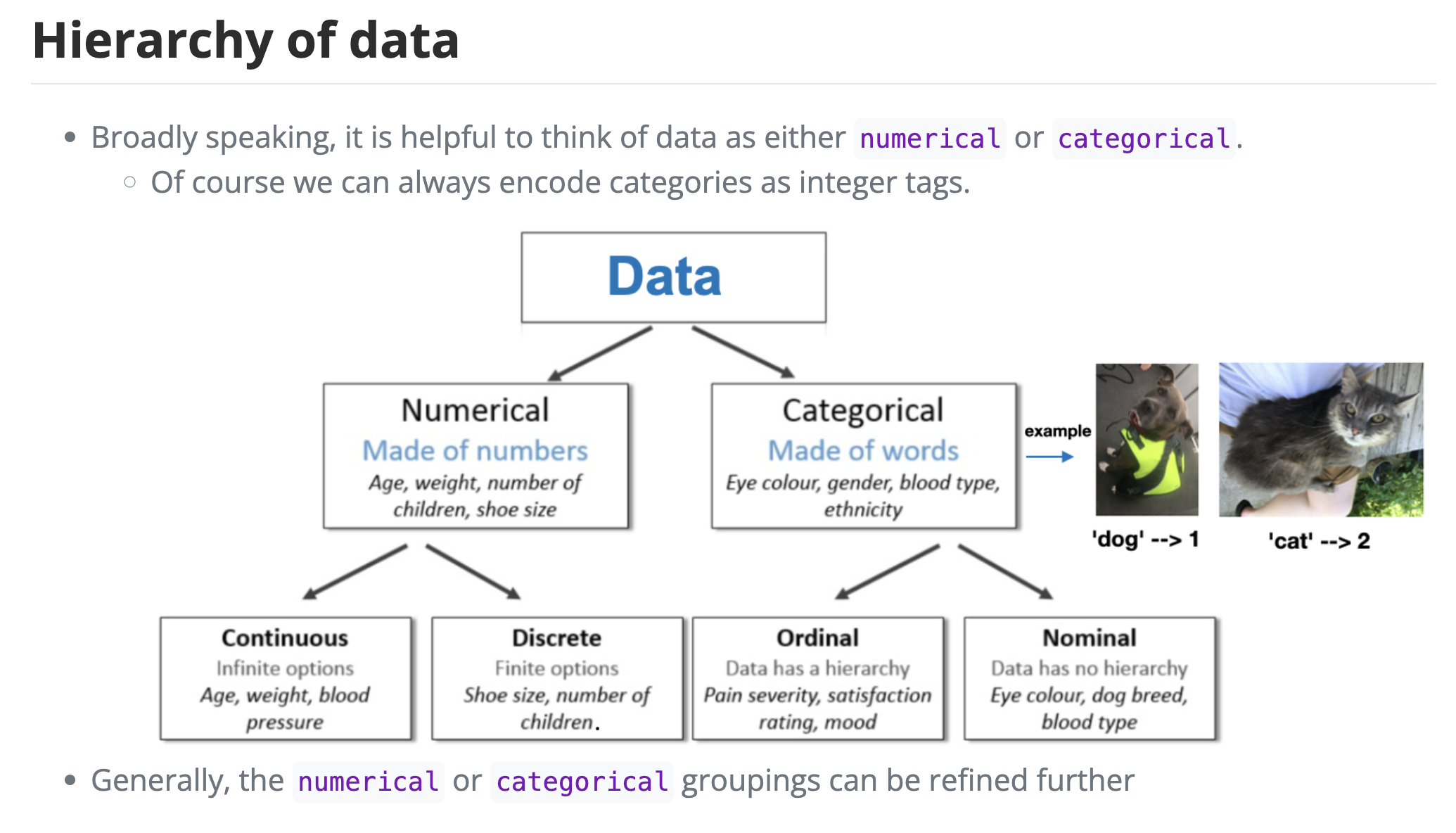
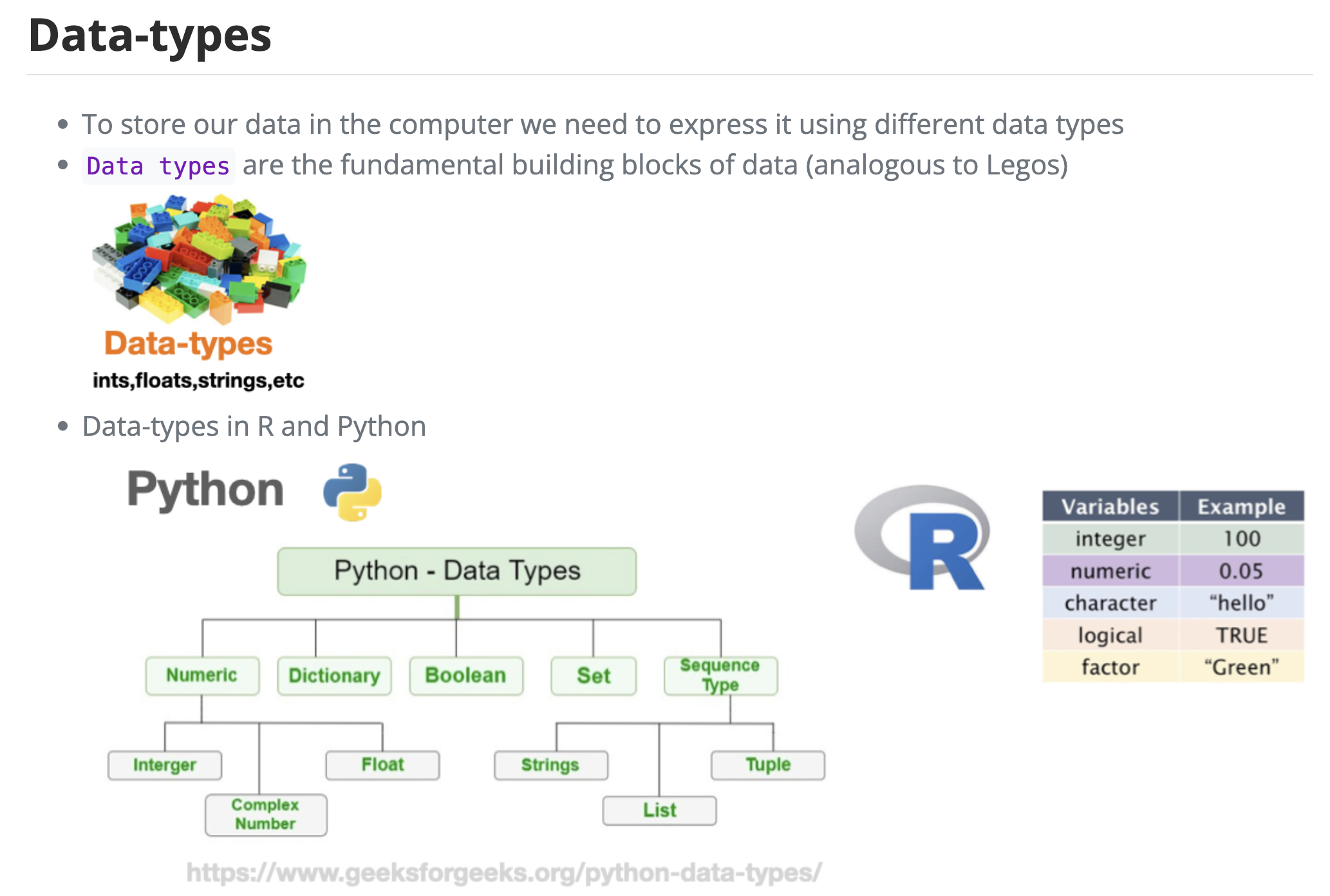
R has a small set of atomic types. Everything else is built from them.
double: real numbers, the default for any number you typeinteger: whole numbers, written with a trailingLcharacter: text, in single or double quoteslogical:TRUEandFALSEcomplexandraw: rarely needed in an intro course
a <- 3.14        # double
b <- 3L          # integer
d <- "hello"     # character
e <- TRUE        # logical

typeof(a)
typeof(b)
typeof(d)
typeof(e)
'double'
'integer'
'character'
'logical'
Inspecting an object
Three questions worth asking about any object you did not create yourself.
typeof(): what is the low-level storage typeclass(): what does R treat this as for dispatch purposesstr(): compact structural summary, the single most useful inspection function
x <- 3.14

typeof(x)       # "double"
class(x)        # "numeric"
length(x)       # 1: there are no scalars in R, only length-1 vectors
str(x)

is.numeric(x)
is.character(x)
'double'
'numeric'
1
num 3.14
TRUE
FALSE
Type conversion
as.numeric(),as.integer(),as.character(),as.logical()convert explicitly- Failed conversions produce
NAand a warning rather than an error as.integer()truncates toward zero; it does not round
as.integer(3.99)         # 3, truncated
as.character(3.14)       # "3.14"
as.numeric("42")         # 42
as.numeric("banana")     # NA with a warning
as.logical(0)            # FALSE
as.numeric(TRUE)         # 1
3
'3.14'
42
Warning message in eval(expr, envir, enclos):
“NAs introduced by coercion”
<NA>
FALSE
1
Special values
NA: missing value, contagious through most calculationsNULL: the empty object, has length zeroNaN: not a number, from undefined arithmeticInfand-Inf: overflow or division by zero
Test with is.na(), never with == NA.
v <- c(1, 2, NA, 4)

mean(v)                    # NA: missingness propagates
mean(v, na.rm = TRUE)      # drop the NA first

is.na(v)                   # element-wise test
0 / 0                      # NaN
1 / 0                      # Inf
<NA>
2.33333333333333
- FALSE
- FALSE
- TRUE
- FALSE
NaN
Inf
Part 2: Data Structures
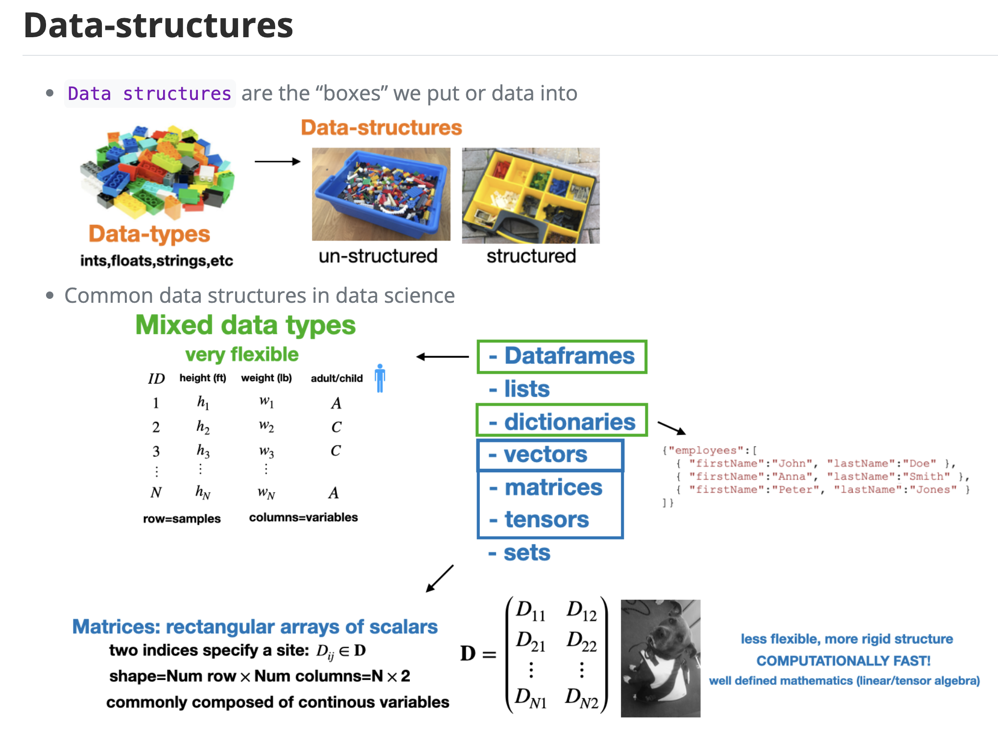
Vectors
The workhorse of R. A vector is an ordered sequence of values, all of the same type.
c()combines values:builds an integer sequenceseq()andrep()build patterned sequences
x <- c(10, 15, 20, 25, 30, 35)
x

1:10
seq(0, 1, by = 0.25)
seq(0, 10, length.out = 5)
rep(c("a", "b"), times = 3)
length(x)- 10
- 15
- 20
- 25
- 30
- 35
- 1
- 2
- 3
- 4
- 5
- 6
- 7
- 8
- 9
- 10
- 0
- 0.25
- 0.5
- 0.75
- 1
- 0
- 2.5
- 5
- 7.5
- 10
- 'a'
- 'b'
- 'a'
- 'b'
- 'a'
- 'b'
6
Indexing vectors
- R indexes from 1, not from 0
- A negative index means “everything except”
- A logical vector selects the positions that are
TRUE
x <- c(10, 15, 20, 25, 30, 35)

x[1]              # first element
x[length(x)]      # last element
x[2:4]            # a contiguous slice
x[c(1, 5)]        # arbitrary positions
x[-1]             # drop the first element
x[x > 20]         # logical subsetting: the key idiom
10
35
- 15
- 20
- 25
- 10
- 30
- 15
- 20
- 25
- 30
- 35
- 25
- 30
- 35
Vectorized operations
Operations apply element-by-element with no loop required. This is the central habit to build in R.
- Shorter vectors are recycled to match longer ones
- Recycling with mismatched lengths is a common source of silent bugs
x <- c(1, 2, 3, 4)

x * 2             # every element doubled
x + x
x^2
sqrt(x)

sum(x); mean(x); max(x); sd(x)- 2
- 4
- 6
- 8
- 2
- 4
- 6
- 8
- 1
- 4
- 9
- 16
- 1
- 1.4142135623731
- 1.73205080756888
- 2
10
2.5
4
1.29099444873581
Named vectors and coercion
- Elements can carry names, accessible by name instead of position
- A vector holds exactly one type; mixing types silently coerces everything upward
- The coercion ladder: logical, then integer, then double, then character
scores <- c(math = 90, art = 75, bio = 88)
scores["art"]

c(1, 2, TRUE)          # logical becomes numeric
c(1, 2, "three")       # everything becomes character
art: 75
- 1
- 2
- 1
- '1'
- '2'
- 'three'
Matrices
A matrix is a vector with a two-dimensional shape attribute.
- Filled column-first by default
- Indexed as
[row, column]; leaving a slot blank keeps that whole dimension
m <- matrix(1:20, nrow = 5, ncol = 4)
m

dim(m)
m[3, 2]        # single element
m[3, ]         # third row
m[, 2]         # second column
t(m) # transpose| 1 | 6 | 11 | 16 |
| 2 | 7 | 12 | 17 |
| 3 | 8 | 13 | 18 |
| 4 | 9 | 14 | 19 |
| 5 | 10 | 15 | 20 |
- 5
- 4
8
- 3
- 8
- 13
- 18
- 6
- 7
- 8
- 9
- 10
| 1 | 2 | 3 | 4 | 5 |
| 6 | 7 | 8 | 9 | 10 |
| 11 | 12 | 13 | 14 | 15 |
| 16 | 17 | 18 | 19 | 20 |
Lists
A list holds elements of different types and different lengths.
[[ ]]or$extracts the element itself[ ]returns a shorter list, not the element
person <- list(name = "Ada", age = 36, scores = c(90, 95, 99))

str(person)
person$name
person[["scores"]]
person$scores[2]
List of 3
$ name : chr "Ada"
$ age : num 36
$ scores: num [1:3] 90 95 99
'Ada'
- 90
- 95
- 99
95
Factors
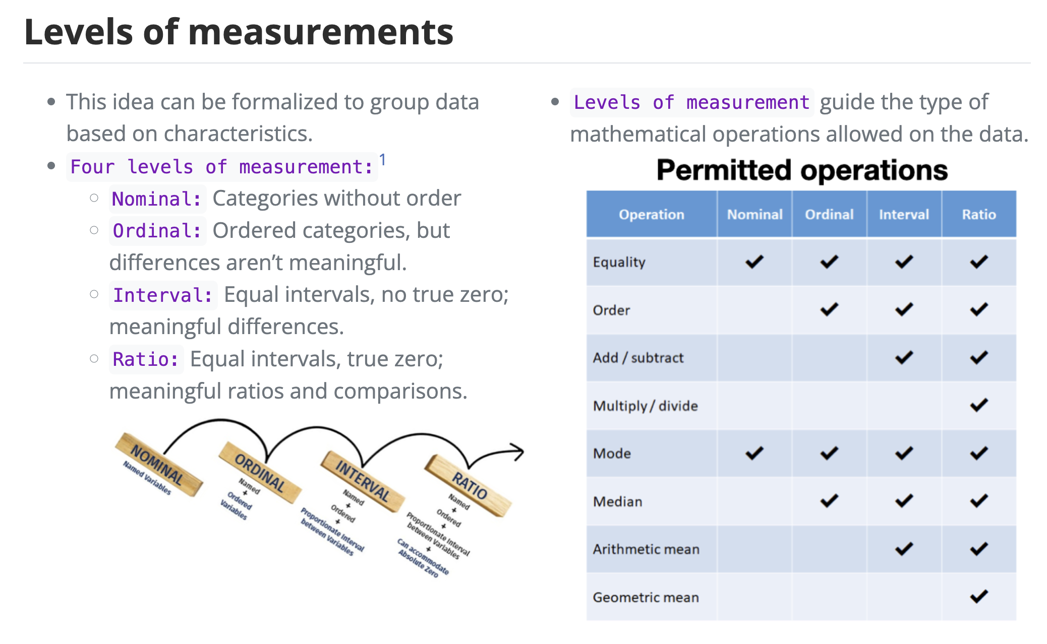
Factors represent categorical data with a fixed set of possible values, called levels.
- Stored as integers with a label lookup table
- Level order controls the order categories appear in tables and plots
sizes <- factor(c("small", "large", "small", "medium"),
                levels = c("small", "medium", "large"))

sizes
levels(sizes)
table(sizes)
as.integer(sizes) # the underlying codes- small
- large
- small
- medium
Levels:
- 'small'
- 'medium'
- 'large'
- 'small'
- 'medium'
- 'large'
sizes
 small medium  large
2 1 1 - 1
- 3
- 1
- 2
Data frames
A data frame is a list of equal-length vectors displayed as a table: rows are observations, columns are variables.
- Each column has its own type
- This is the structure nearly all real analysis uses
df <- data.frame(
  id     = c(10, 20, 30, 40),
  color  = c("red", "white", "red", NA),
  passed = c(TRUE, TRUE, TRUE, FALSE)
)

df
str(df)
dim(df)
names(df)| id | color | passed |
|---|---|---|
| <dbl> | <chr> | <lgl> |
| 10 | red | TRUE |
| 20 | white | TRUE |
| 30 | red | TRUE |
| 40 | NA | FALSE |
'data.frame':   4 obs. of  3 variables:
 $ id    : num  10 20 30 40
 $ color : chr  "red" "white" "red" NA
$ passed: logi TRUE TRUE TRUE FALSE- 4
- 3
- 'id'
- 'color'
- 'passed'
Working with data frames
$pulls a single column out as a vectordf[rows, columns]subsets in two dimensionshead(),summary(), andstr()are the first three things to run on any new dataset
df$id
df[df$passed, ]           # rows where passed is TRUE
df[, c("id", "color")]    # selected columns

head(mtcars)              # a built-in dataset
summary(mtcars$mpg)- 10
- 20
- 30
- 40
| id | color | passed | |
|---|---|---|---|
| <dbl> | <chr> | <lgl> | |
| 1 | 10 | red | TRUE |
| 2 | 20 | white | TRUE |
| 3 | 30 | red | TRUE |
| id | color |
|---|---|
| <dbl> | <chr> |
| 10 | red |
| 20 | white |
| 30 | red |
| 40 | NA |
| mpg | cyl | disp | hp | drat | wt | qsec | vs | am | gear | carb | |
|---|---|---|---|---|---|---|---|---|---|---|---|
| <dbl> | <dbl> | <dbl> | <dbl> | <dbl> | <dbl> | <dbl> | <dbl> | <dbl> | <dbl> | <dbl> | |
| Mazda RX4 | 21.0 | 6 | 160 | 110 | 3.90 | 2.620 | 16.46 | 0 | 1 | 4 | 4 |
| Mazda RX4 Wag | 21.0 | 6 | 160 | 110 | 3.90 | 2.875 | 17.02 | 0 | 1 | 4 | 4 |
| Datsun 710 | 22.8 | 4 | 108 | 93 | 3.85 | 2.320 | 18.61 | 1 | 1 | 4 | 1 |
| Hornet 4 Drive | 21.4 | 6 | 258 | 110 | 3.08 | 3.215 | 19.44 | 1 | 0 | 3 | 1 |
| Hornet Sportabout | 18.7 | 8 | 360 | 175 | 3.15 | 3.440 | 17.02 | 0 | 0 | 3 | 2 |
| Valiant | 18.1 | 6 | 225 | 105 | 2.76 | 3.460 | 20.22 | 1 | 0 | 3 | 1 |
   Min. 1st Qu.  Median    Mean 3rd Qu.    Max.
  10.40   15.43   19.20   20.09   22.80   33.90
Part 3: Control Flow and Functions
Conditionals
if/else if/elsetakes a singleTRUEorFALSEifelse()is the vectorized version, applied element-wise across a vector
score <- 85

if (score >= 90) {
  print("A")
} else if (score >= 80) {
  print("B")
} else {
  print("C")
}

scores <- c(95, 85, 60)
ifelse(scores >= 80, "pass", "fail")    # vectorized
[1] "B"- 'pass'
- 'pass'
- 'fail'
For loops
for (item in sequence)iterates over any vector or listseq_along(x)is safer than1:length(x), which misbehaves on empty vectors- Preallocate the output vector rather than growing it inside the loop
for (i in 1:5) {
  cat("i =", i, " i^2 =", i^2, "\n")
}

# preallocate, then fill
squares <- numeric(5)
for (i in seq_along(squares)) {
  squares[i] <- i^2
}
squares
i = 1 i^2 = 1
i = 2 i^2 = 4
i = 3 i^2 = 9
i = 4 i^2 = 16
i = 5 i^2 = 25 - 1
- 4
- 9
- 16
- 25
While loops
- Repeats while a condition stays
TRUE - Use when the number of iterations is not known in advance
- Make sure something inside the loop can eventually flip the condition
i <- 1
while (i <= 5) {
  print(i)
  i <- i + 1
}
[1] 1
[1] 2
[1] 3
[1] 4
[1] 5Writing functions
function(arguments) { body }, assigned to a name- The last expression evaluated is returned automatically;
return()is optional - Arguments can carry default values
summarize_vec <- function(x, digits = 2) {
  round(c(mean = mean(x), sd = sd(x), n = length(x)), digits)
}

v <- c(4, 8, 15, 16, 23, 42)
summarize_vec(v)
summarize_vec(v, digits = 4)- mean
- 18
- sd
- 13.49
- n
- 6
- mean
- 18
- sd
- 13.4907
- n
- 6
The apply family
Idiomatic R replaces most loops with a function applied across a structure.
sapply(): apply to each element, simplify the result to a vectorlapply(): same, but always returns a listapply(): apply along the rows (1) or columns (2) of a matrix
sapply(1:5, function(i) i^2)

apply(m, 2, sum)      # column sums of the matrix from earlier
apply(m, 1, max)      # row maxima

sapply(mtcars[, c("mpg", "hp", "wt")], mean)- 1
- 4
- 9
- 16
- 25
- 15
- 40
- 65
- 90
- 16
- 17
- 18
- 19
- 20
- mpg
- 20.090625
- hp
- 146.6875
- wt
- 3.21725
Getting unstuck
?meanorhelp(mean)opens the documentation, including runnable examplesstr(x)when a result surprises you: the problem is almost always the typels()lists everything currently defined in your environment- Read the error message literally, then search it verbatim
a <- 1; b <- "two"
ls()

# ?mean        # uncomment to open help
str(mtcars)- 'a'
- 'b'
- 'd'
- 'df'
- 'e'
- 'i'
- 'long'
- 'm'
- 'person'
- 'score'
- 'scores'
- 'sizes'
- 'squares'
- 'summarize_vec'
- 'v'
- 'x'
- 'y'
- 'z'
'data.frame':   32 obs. of  11 variables:
 $ mpg : num  21 21 22.8 21.4 18.7 18.1 14.3 24.4 22.8 19.2 ...
 $ cyl : num  6 6 4 6 8 6 8 4 4 6 ...
 $ disp: num  160 160 108 258 360 ...
 $ hp  : num  110 110 93 110 175 105 245 62 95 123 ...
 $ drat: num  3.9 3.9 3.85 3.08 3.15 2.76 3.21 3.69 3.92 3.92 ...
 $ wt  : num  2.62 2.88 2.32 3.21 3.44 ...
 $ qsec: num  16.5 17 18.6 19.4 17 ...
 $ vs  : num  0 0 1 1 0 1 0 1 1 1 ...
 $ am  : num  1 1 1 0 0 0 0 0 0 0 ...
 $ gear: num  4 4 4 3 3 3 3 4 4 4 ...
 $ carb: num  4 4 1 1 2 1 4 2 2 4 ...
Part 4: The Tidyverse
What the tidyverse is
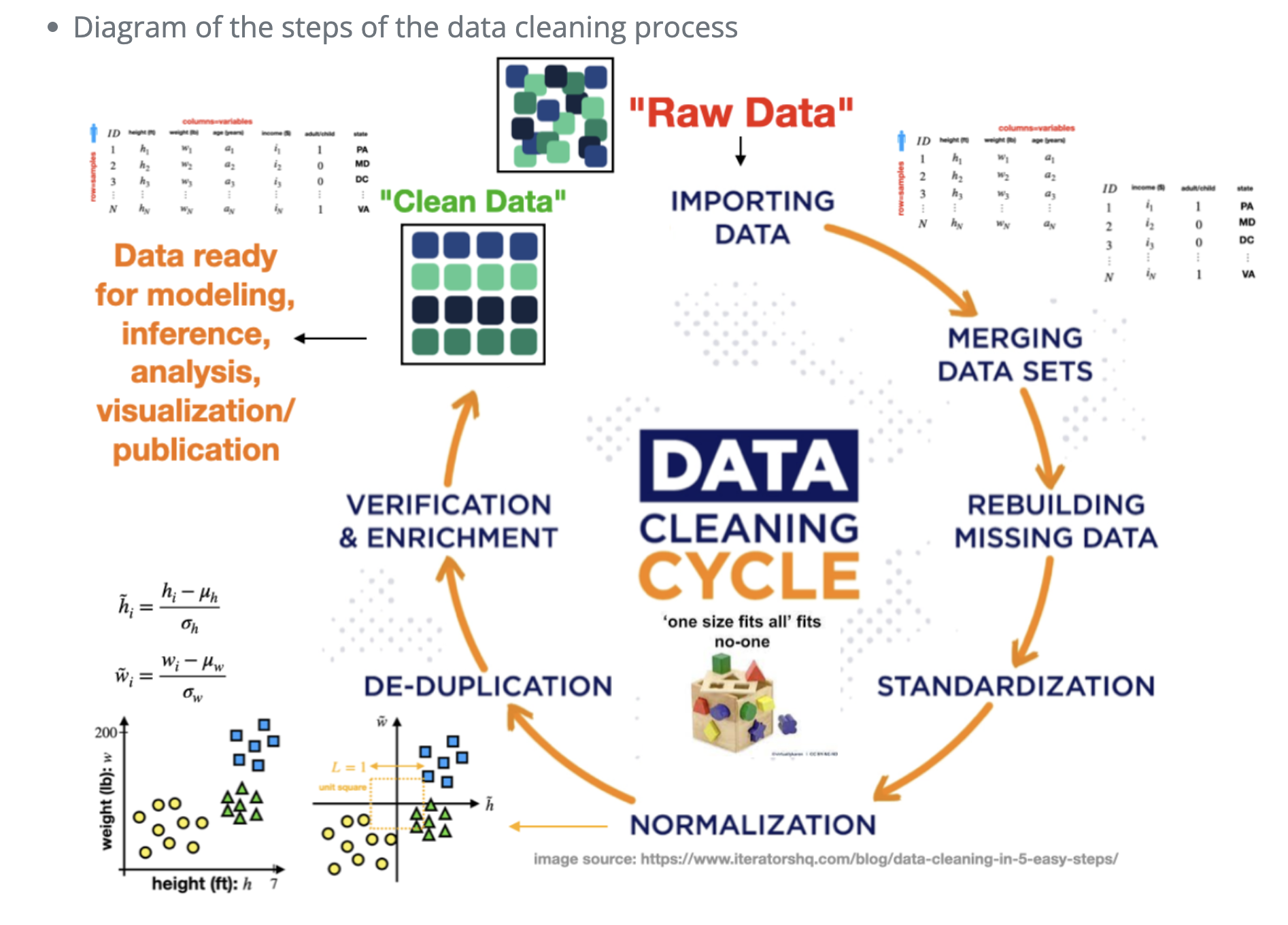
A collection of packages sharing a common design, loaded together with one call.
dplyr: data manipulation verbsggplot2: visualizationtidyr: reshaping between wide and long formreadr: fast file importtibble,stringr,forcats,purrr: tables, strings, factors, functional tools
Install once, load every session.
# install.packages("tidyverse")   # run once, then comment out
library(tidyverse)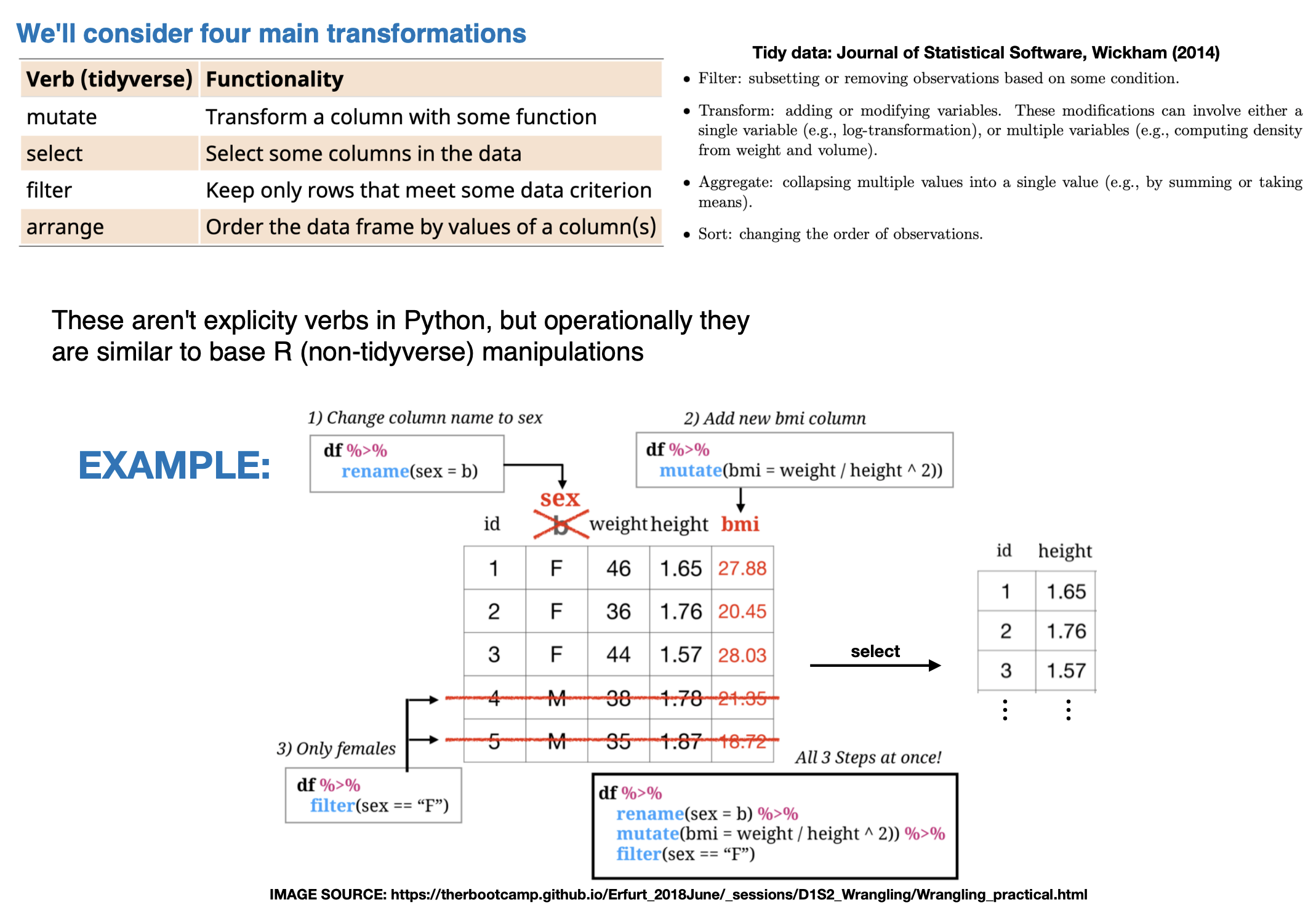
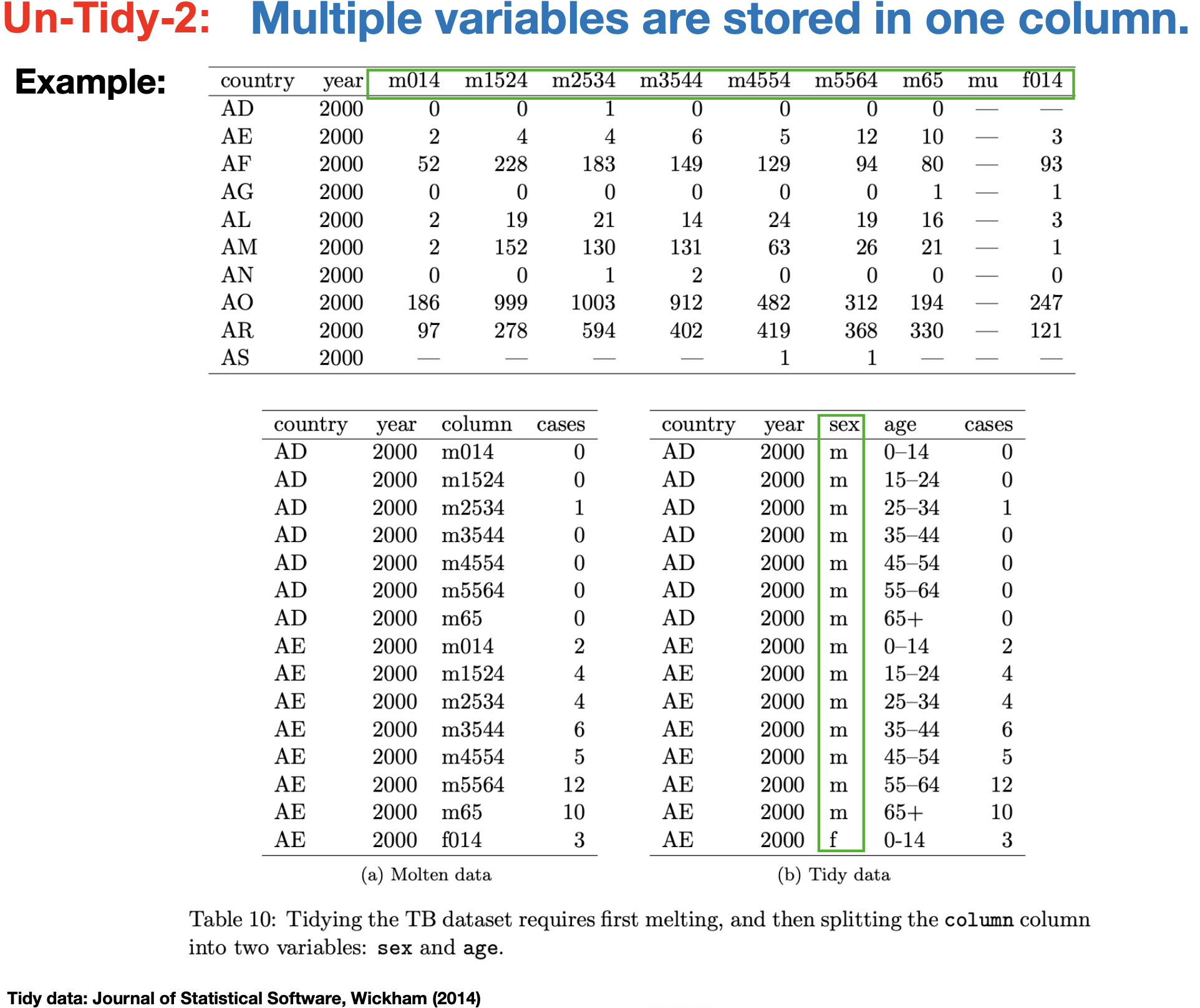
Tidy data
One rule governs everything downstream.
- Each variable is a column
- Each observation is a row
- Each cell is a single value
Data in this shape works directly with every tidyverse function.
mpg          # a tibble shipped with ggplot2: 234 car models
glimpse(mpg) # the tidyverse counterpart to str()| manufacturer | model | displ | year | cyl | trans | drv | cty | hwy | fl | class |
|---|---|---|---|---|---|---|---|---|---|---|
| <chr> | <chr> | <dbl> | <int> | <int> | <chr> | <chr> | <int> | <int> | <chr> | <chr> |
| audi | a4 | 1.8 | 1999 | 4 | auto(l5) | f | 18 | 29 | p | compact |
| audi | a4 | 1.8 | 1999 | 4 | manual(m5) | f | 21 | 29 | p | compact |
| audi | a4 | 2.0 | 2008 | 4 | manual(m6) | f | 20 | 31 | p | compact |
| audi | a4 | 2.0 | 2008 | 4 | auto(av) | f | 21 | 30 | p | compact |
| audi | a4 | 2.8 | 1999 | 6 | auto(l5) | f | 16 | 26 | p | compact |
| audi | a4 | 2.8 | 1999 | 6 | manual(m5) | f | 18 | 26 | p | compact |
| audi | a4 | 3.1 | 2008 | 6 | auto(av) | f | 18 | 27 | p | compact |
| audi | a4 quattro | 1.8 | 1999 | 4 | manual(m5) | 4 | 18 | 26 | p | compact |
| audi | a4 quattro | 1.8 | 1999 | 4 | auto(l5) | 4 | 16 | 25 | p | compact |
| audi | a4 quattro | 2.0 | 2008 | 4 | manual(m6) | 4 | 20 | 28 | p | compact |
| audi | a4 quattro | 2.0 | 2008 | 4 | auto(s6) | 4 | 19 | 27 | p | compact |
| audi | a4 quattro | 2.8 | 1999 | 6 | auto(l5) | 4 | 15 | 25 | p | compact |
| audi | a4 quattro | 2.8 | 1999 | 6 | manual(m5) | 4 | 17 | 25 | p | compact |
| audi | a4 quattro | 3.1 | 2008 | 6 | auto(s6) | 4 | 17 | 25 | p | compact |
| audi | a4 quattro | 3.1 | 2008 | 6 | manual(m6) | 4 | 15 | 25 | p | compact |
| audi | a6 quattro | 2.8 | 1999 | 6 | auto(l5) | 4 | 15 | 24 | p | midsize |
| audi | a6 quattro | 3.1 | 2008 | 6 | auto(s6) | 4 | 17 | 25 | p | midsize |
| audi | a6 quattro | 4.2 | 2008 | 8 | auto(s6) | 4 | 16 | 23 | p | midsize |
| chevrolet | c1500 suburban 2wd | 5.3 | 2008 | 8 | auto(l4) | r | 14 | 20 | r | suv |
| chevrolet | c1500 suburban 2wd | 5.3 | 2008 | 8 | auto(l4) | r | 11 | 15 | e | suv |
| chevrolet | c1500 suburban 2wd | 5.3 | 2008 | 8 | auto(l4) | r | 14 | 20 | r | suv |
| chevrolet | c1500 suburban 2wd | 5.7 | 1999 | 8 | auto(l4) | r | 13 | 17 | r | suv |
| chevrolet | c1500 suburban 2wd | 6.0 | 2008 | 8 | auto(l4) | r | 12 | 17 | r | suv |
| chevrolet | corvette | 5.7 | 1999 | 8 | manual(m6) | r | 16 | 26 | p | 2seater |
| chevrolet | corvette | 5.7 | 1999 | 8 | auto(l4) | r | 15 | 23 | p | 2seater |
| chevrolet | corvette | 6.2 | 2008 | 8 | manual(m6) | r | 16 | 26 | p | 2seater |
| chevrolet | corvette | 6.2 | 2008 | 8 | auto(s6) | r | 15 | 25 | p | 2seater |
| chevrolet | corvette | 7.0 | 2008 | 8 | manual(m6) | r | 15 | 24 | p | 2seater |
| chevrolet | k1500 tahoe 4wd | 5.3 | 2008 | 8 | auto(l4) | 4 | 14 | 19 | r | suv |
| chevrolet | k1500 tahoe 4wd | 5.3 | 2008 | 8 | auto(l4) | 4 | 11 | 14 | e | suv |
| ⋮ | ⋮ | ⋮ | ⋮ | ⋮ | ⋮ | ⋮ | ⋮ | ⋮ | ⋮ | ⋮ |
| toyota | toyota tacoma 4wd | 3.4 | 1999 | 6 | auto(l4) | 4 | 15 | 19 | r | pickup |
| toyota | toyota tacoma 4wd | 4.0 | 2008 | 6 | manual(m6) | 4 | 15 | 18 | r | pickup |
| toyota | toyota tacoma 4wd | 4.0 | 2008 | 6 | auto(l5) | 4 | 16 | 20 | r | pickup |
| volkswagen | gti | 2.0 | 1999 | 4 | manual(m5) | f | 21 | 29 | r | compact |
| volkswagen | gti | 2.0 | 1999 | 4 | auto(l4) | f | 19 | 26 | r | compact |
| volkswagen | gti | 2.0 | 2008 | 4 | manual(m6) | f | 21 | 29 | p | compact |
| volkswagen | gti | 2.0 | 2008 | 4 | auto(s6) | f | 22 | 29 | p | compact |
| volkswagen | gti | 2.8 | 1999 | 6 | manual(m5) | f | 17 | 24 | r | compact |
| volkswagen | jetta | 1.9 | 1999 | 4 | manual(m5) | f | 33 | 44 | d | compact |
| volkswagen | jetta | 2.0 | 1999 | 4 | manual(m5) | f | 21 | 29 | r | compact |
| volkswagen | jetta | 2.0 | 1999 | 4 | auto(l4) | f | 19 | 26 | r | compact |
| volkswagen | jetta | 2.0 | 2008 | 4 | auto(s6) | f | 22 | 29 | p | compact |
| volkswagen | jetta | 2.0 | 2008 | 4 | manual(m6) | f | 21 | 29 | p | compact |
| volkswagen | jetta | 2.5 | 2008 | 5 | auto(s6) | f | 21 | 29 | r | compact |
| volkswagen | jetta | 2.5 | 2008 | 5 | manual(m5) | f | 21 | 29 | r | compact |
| volkswagen | jetta | 2.8 | 1999 | 6 | auto(l4) | f | 16 | 23 | r | compact |
| volkswagen | jetta | 2.8 | 1999 | 6 | manual(m5) | f | 17 | 24 | r | compact |
| volkswagen | new beetle | 1.9 | 1999 | 4 | manual(m5) | f | 35 | 44 | d | subcompact |
| volkswagen | new beetle | 1.9 | 1999 | 4 | auto(l4) | f | 29 | 41 | d | subcompact |
| volkswagen | new beetle | 2.0 | 1999 | 4 | manual(m5) | f | 21 | 29 | r | subcompact |
| volkswagen | new beetle | 2.0 | 1999 | 4 | auto(l4) | f | 19 | 26 | r | subcompact |
| volkswagen | new beetle | 2.5 | 2008 | 5 | manual(m5) | f | 20 | 28 | r | subcompact |
| volkswagen | new beetle | 2.5 | 2008 | 5 | auto(s6) | f | 20 | 29 | r | subcompact |
| volkswagen | passat | 1.8 | 1999 | 4 | manual(m5) | f | 21 | 29 | p | midsize |
| volkswagen | passat | 1.8 | 1999 | 4 | auto(l5) | f | 18 | 29 | p | midsize |
| volkswagen | passat | 2.0 | 2008 | 4 | auto(s6) | f | 19 | 28 | p | midsize |
| volkswagen | passat | 2.0 | 2008 | 4 | manual(m6) | f | 21 | 29 | p | midsize |
| volkswagen | passat | 2.8 | 1999 | 6 | auto(l5) | f | 16 | 26 | p | midsize |
| volkswagen | passat | 2.8 | 1999 | 6 | manual(m5) | f | 18 | 26 | p | midsize |
| volkswagen | passat | 3.6 | 2008 | 6 | auto(s6) | f | 17 | 26 | p | midsize |
Rows: 234
Columns: 11
$ manufacturer <chr> "audi", "audi", "audi", "audi", "audi", "audi", "audi", "…
$ model        <chr> "a4", "a4", "a4", "a4", "a4", "a4", "a4", "a4 quattro", "…
$ displ        <dbl> 1.8, 1.8, 2.0, 2.0, 2.8, 2.8, 3.1, 1.8, 1.8, 2.0, 2.0, 2.…
$ year         <int> 1999, 1999, 2008, 2008, 1999, 1999, 2008, 1999, 1999, 200…
$ cyl          <int> 4, 4, 4, 4, 6, 6, 6, 4, 4, 4, 4, 6, 6, 6, 6, 6, 6, 8, 8, …
$ trans        <chr> "auto(l5)", "manual(m5)", "manual(m6)", "auto(av)", "auto…
$ drv          <chr> "f", "f", "f", "f", "f", "f", "f", "4", "4", "4", "4", "4…
$ cty          <int> 18, 21, 20, 21, 16, 18, 18, 18, 16, 20, 19, 15, 17, 17, 1…
$ hwy          <int> 29, 29, 31, 30, 26, 26, 27, 26, 25, 28, 27, 25, 25, 25, 2…
$ fl           <chr> "p", "p", "p", "p", "p", "p", "p", "p", "p", "p", "p", "p…
$ class        <chr> "compact", "compact", "compact", "compact", "compact", "c…
The pipe
|> passes the result on the left into the first argument of the function on the right.
- Turns nested calls into a readable top-to-bottom sequence
%>%from magrittr is the older form and behaves the same way here
# without the pipe
head(filter(mpg, cyl == 4), 3)

# with the pipe: read it as "take mpg, then filter, then take the head"
mpg |>
  filter(cyl == 4) |>
head(3)| manufacturer | model | displ | year | cyl | trans | drv | cty | hwy | fl | class |
|---|---|---|---|---|---|---|---|---|---|---|
| <chr> | <chr> | <dbl> | <int> | <int> | <chr> | <chr> | <int> | <int> | <chr> | <chr> |
| audi | a4 | 1.8 | 1999 | 4 | auto(l5) | f | 18 | 29 | p | compact |
| audi | a4 | 1.8 | 1999 | 4 | manual(m5) | f | 21 | 29 | p | compact |
| audi | a4 | 2.0 | 2008 | 4 | manual(m6) | f | 20 | 31 | p | compact |
| manufacturer | model | displ | year | cyl | trans | drv | cty | hwy | fl | class |
|---|---|---|---|---|---|---|---|---|---|---|
| <chr> | <chr> | <dbl> | <int> | <int> | <chr> | <chr> | <int> | <int> | <chr> | <chr> |
| audi | a4 | 1.8 | 1999 | 4 | auto(l5) | f | 18 | 29 | p | compact |
| audi | a4 | 1.8 | 1999 | 4 | manual(m5) | f | 21 | 29 | p | compact |
| audi | a4 | 2.0 | 2008 | 4 | manual(m6) | f | 20 | 31 | p | compact |
The core dplyr verbs
Five functions cover most day-to-day data manipulation.
filter(): keep rows matching a conditionselect(): keep columnsmutate(): add or modify columnsarrange(): sort rows,desc()for descendingsummarize(): collapse many rows into one
mpg |>
  filter(class == "compact") |>
  select(manufacturer, model, displ, hwy) |>
  mutate(km_per_liter = hwy * 0.425) |>
  arrange(desc(hwy)) |>
head(5)| manufacturer | model | displ | hwy | km_per_liter |
|---|---|---|---|---|
| <chr> | <chr> | <dbl> | <int> | <dbl> |
| volkswagen | jetta | 1.9 | 44 | 18.700 |
| toyota | corolla | 1.8 | 37 | 15.725 |
| toyota | corolla | 1.8 | 35 | 14.875 |
| toyota | corolla | 1.8 | 35 | 14.875 |
| toyota | corolla | 1.8 | 33 | 14.025 |
Group and summarize
group_by() splits the data, summarize() collapses each group, and the result is one row per group.
- This single pattern replaces most of what pivot tables do
n()counts rows within the current group
mpg |>
  group_by(class) |>
  summarize(
    n        = n(),
    mean_hwy = mean(hwy),
    mean_cty = mean(cty)
  ) |>
arrange(desc(mean_hwy))| class | n | mean_hwy | mean_cty |
|---|---|---|---|
| <chr> | <int> | <dbl> | <dbl> |
| compact | 47 | 28.29787 | 20.12766 |
| subcompact | 35 | 28.14286 | 20.37143 |
| midsize | 41 | 27.29268 | 18.75610 |
| 2seater | 5 | 24.80000 | 15.40000 |
| minivan | 11 | 22.36364 | 15.81818 |
| suv | 62 | 18.12903 | 13.50000 |
| pickup | 33 | 16.87879 | 13.00000 |
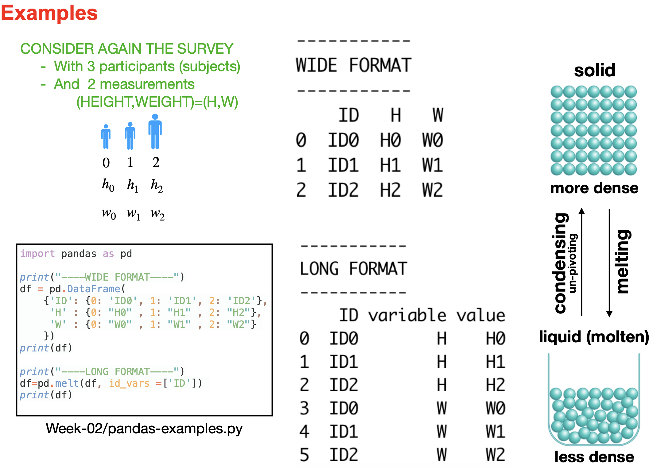
Reshaping with tidyr
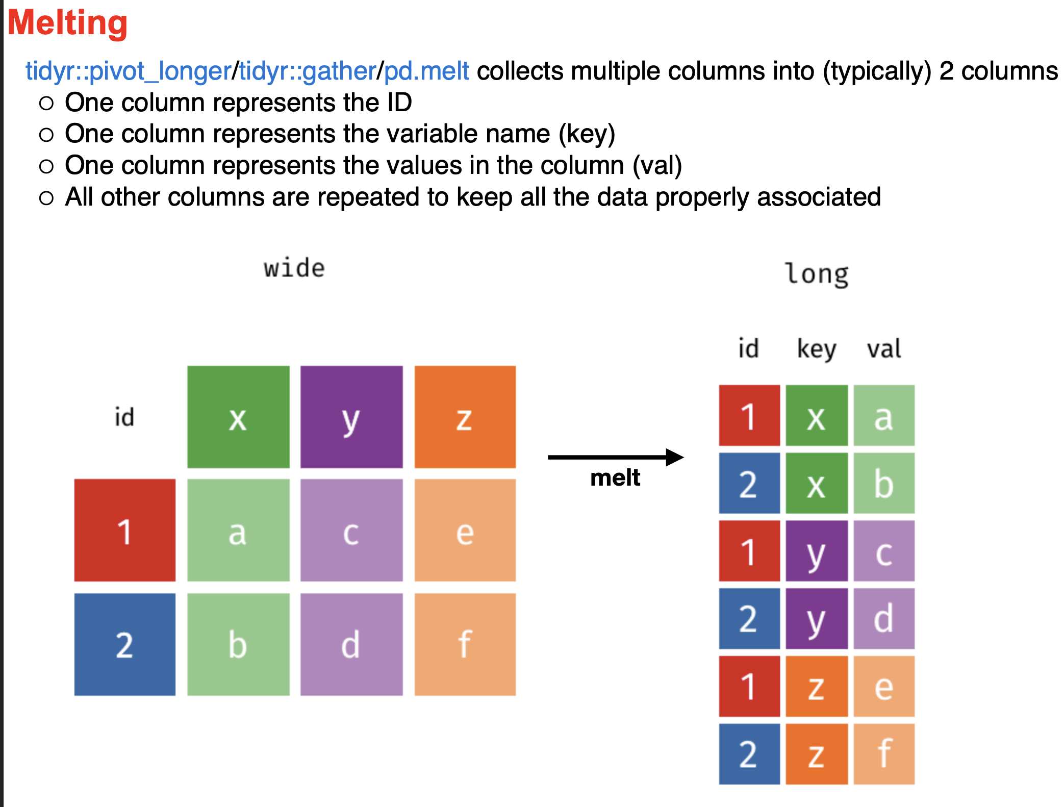
pivot_longer()turns wide data into long data, which is what plotting functions expectpivot_wider()reverses it
long <- mpg |>
  select(model, cty, hwy) |>
  pivot_longer(cols = c(cty, hwy),
               names_to  = "measure",
               values_to = "mpg")

head(long)| model | measure | mpg |
|---|---|---|
| <chr> | <chr> | <int> |
| a4 | cty | 18 |
| a4 | hwy | 29 |
| a4 | cty | 21 |
| a4 | hwy | 29 |
| a4 | cty | 20 |
| a4 | hwy | 31 |