Computational Skills: General improvement in your underlying computational and programming skills
Ecosystem Familiarity: Broad familiarity with the Python and R ecosystems and data visualization libraries, including a fundamental, introductory understanding of what these libraries are doing under the hood
Data Structures: Better understanding of common data structures used in data science (networks, images, text, statistical distributions, etc.)
Visualization Choice: Choosing the correct visualization for the right task (avoid plotting for plotting’s sake)
Generation of professional publication-quality plots: Creation of graphics suitable for inclusion in peer-reviewed publications
Python Proficiency: Deeper exposure to Python and increased general familiarity with the language
Communication: Improvement in general storytelling and communication skills
Data Literacy: Improved numeric and data literacy, and the ability to critically evaluate plots (i.e., better “BS” detection)
Responsible Ai literacy: Try to influence you to adopt AI in a responsible yet productive manner
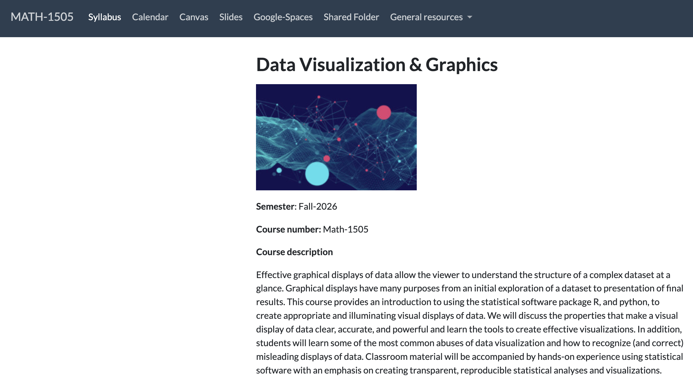
Course website
Lets take a tour of the course website, deliverables, and syllabus!
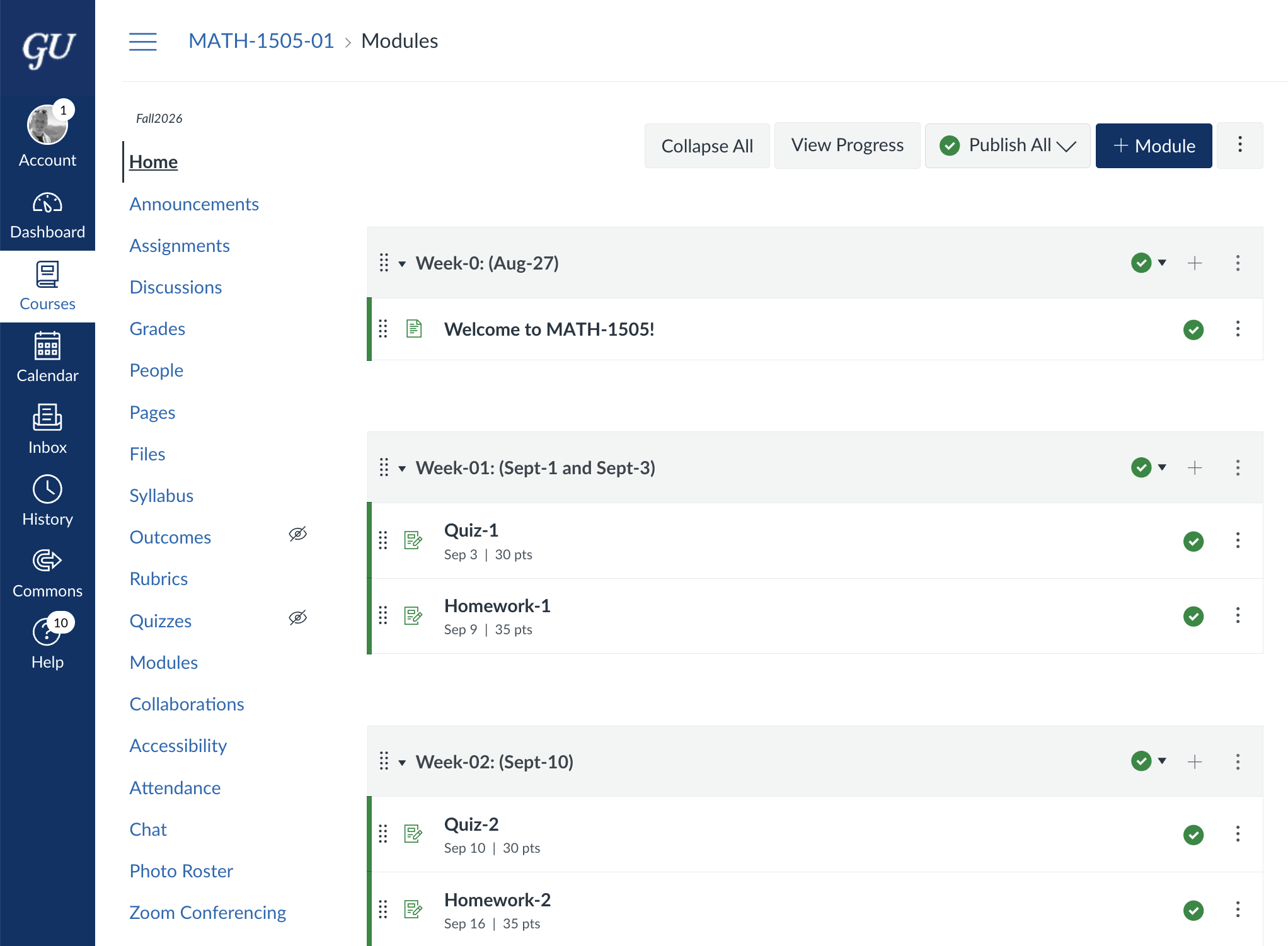
Canvas
Lets take a tour of Canvas!
Word of Advice:
Mathematics is the language of modern technology and science, from LLMs to biology to nuclear physics—so learn the language.
As long as you stay in STEM, you will NEVER regret learning statistics, linear algebra, and calculus at a deeper level.
Learning math is a lifelong journey that is never complete. Each pass gives you deeper understanding and a new perspective.
In short... embrace your inner nerd
Data
Overview
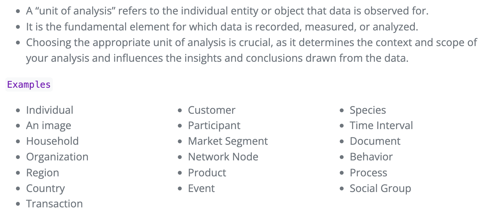
Unit of analysis
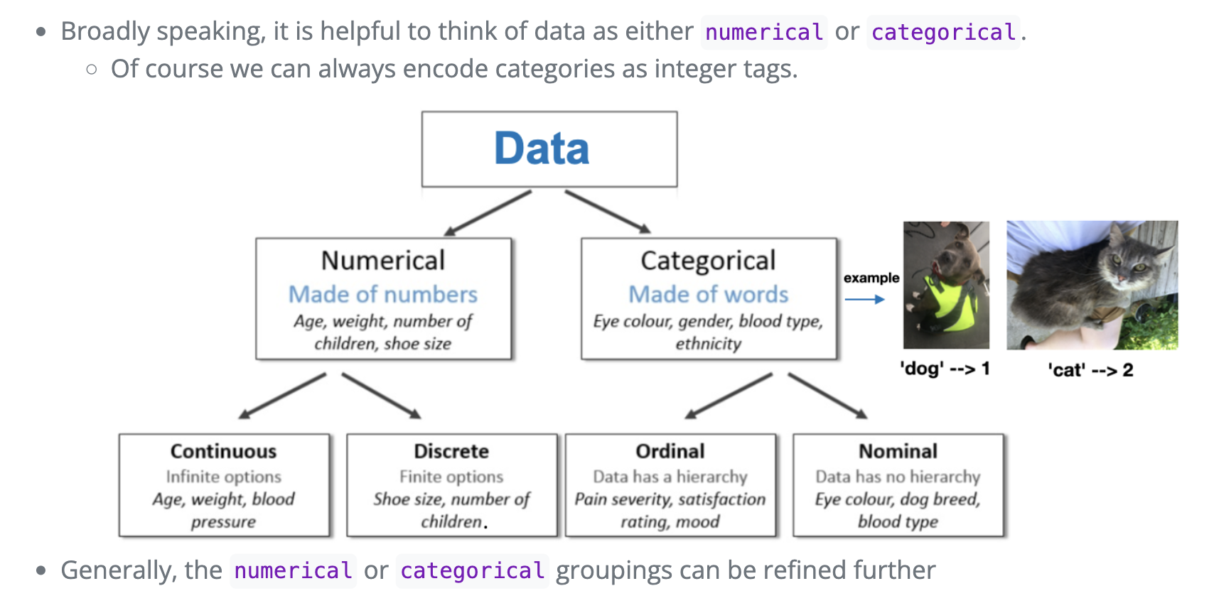
Hierarchy of data
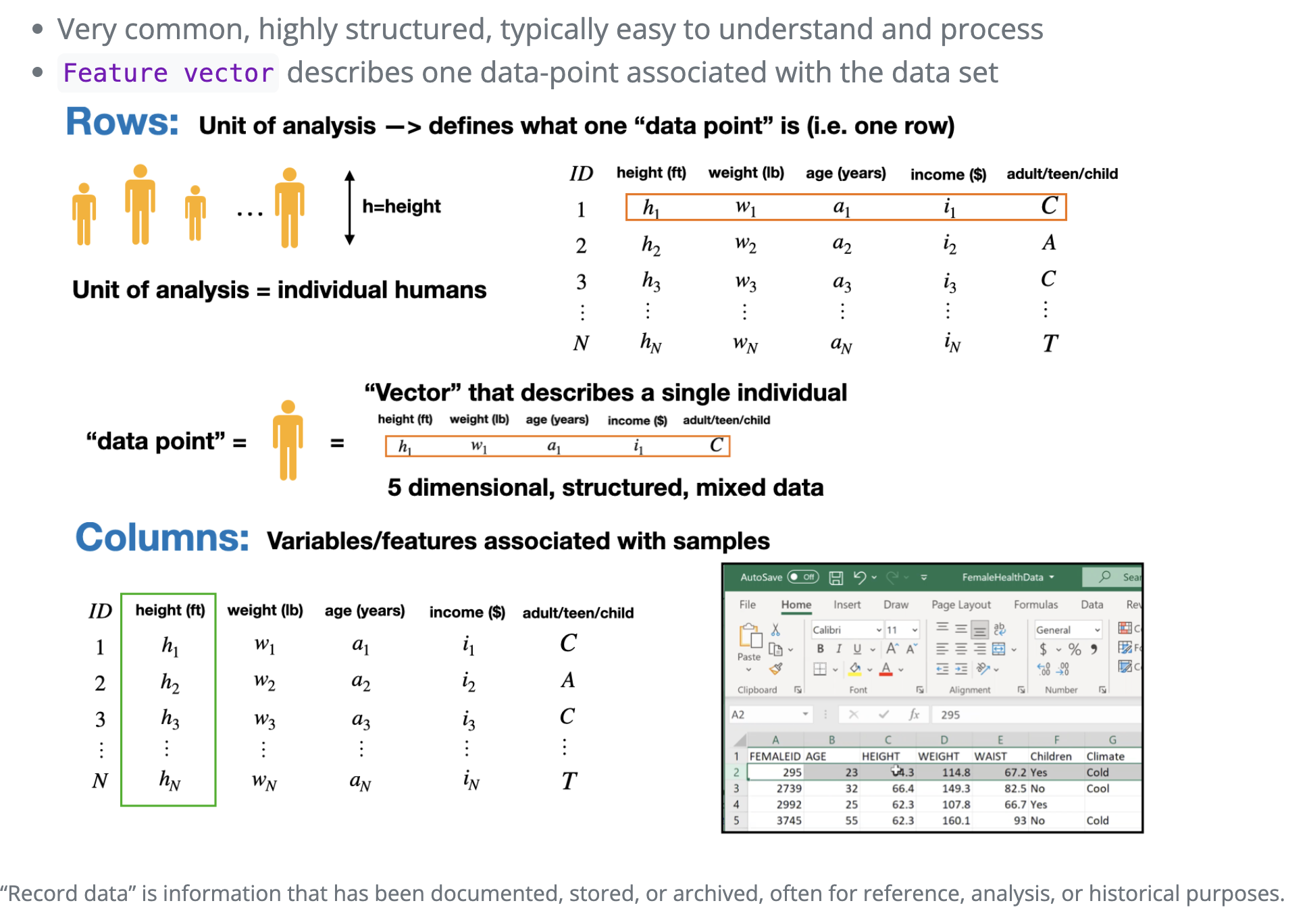
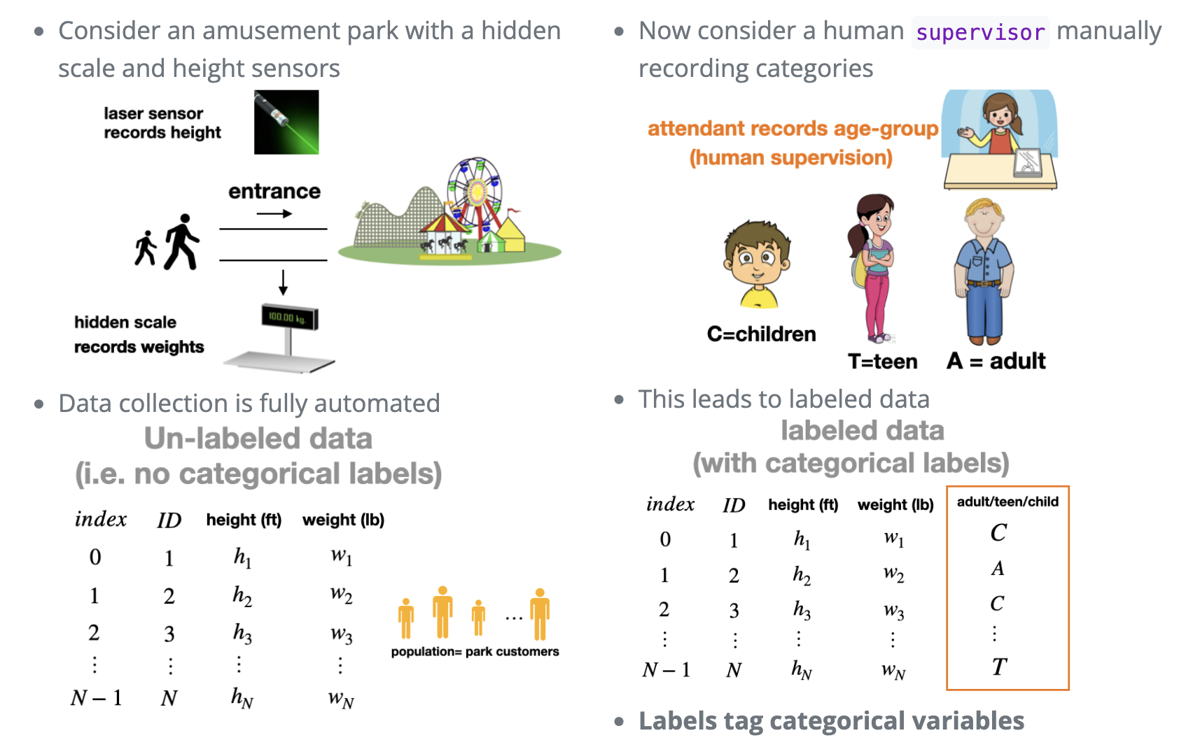
Tabular Data
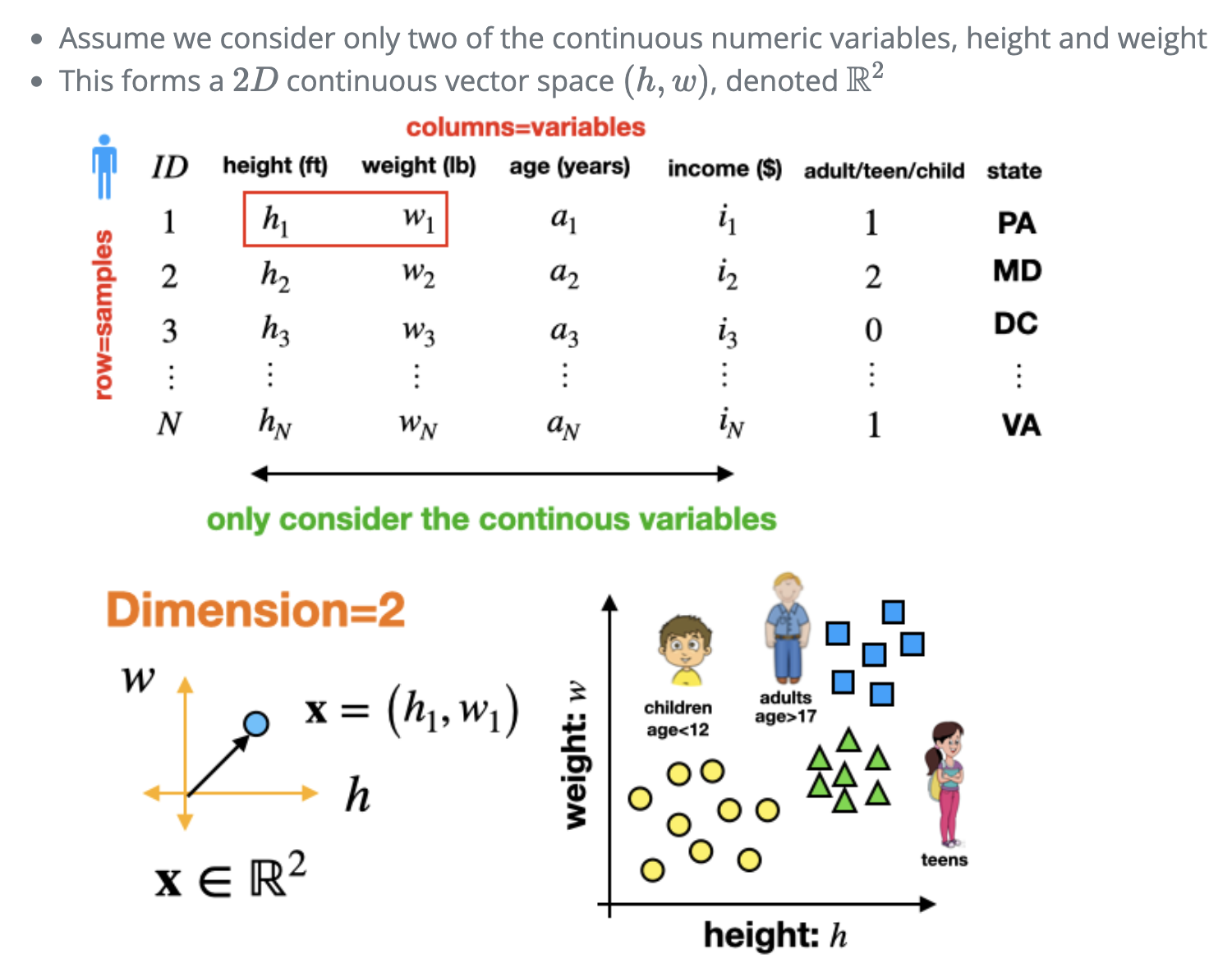
Continuous variables
Labeling and categories
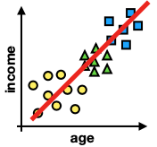
Example: Two dimensional data
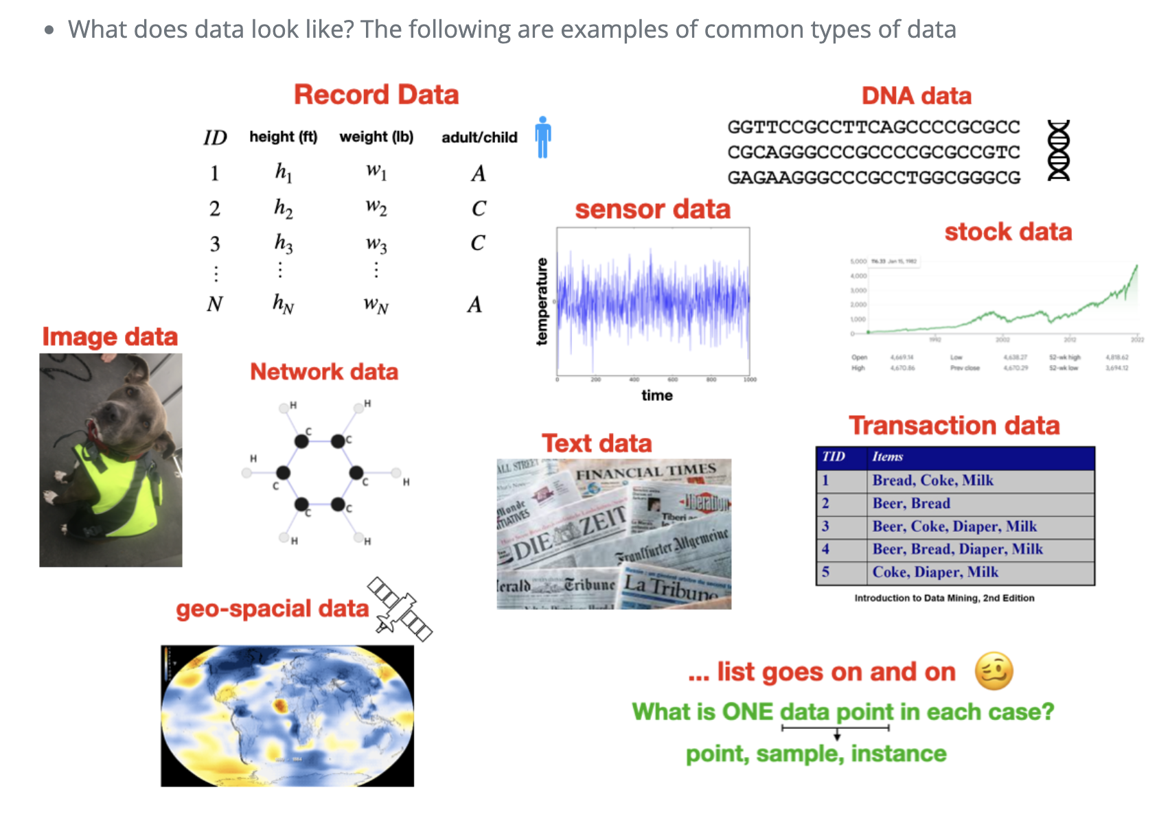
Common types of data
Tabular Data
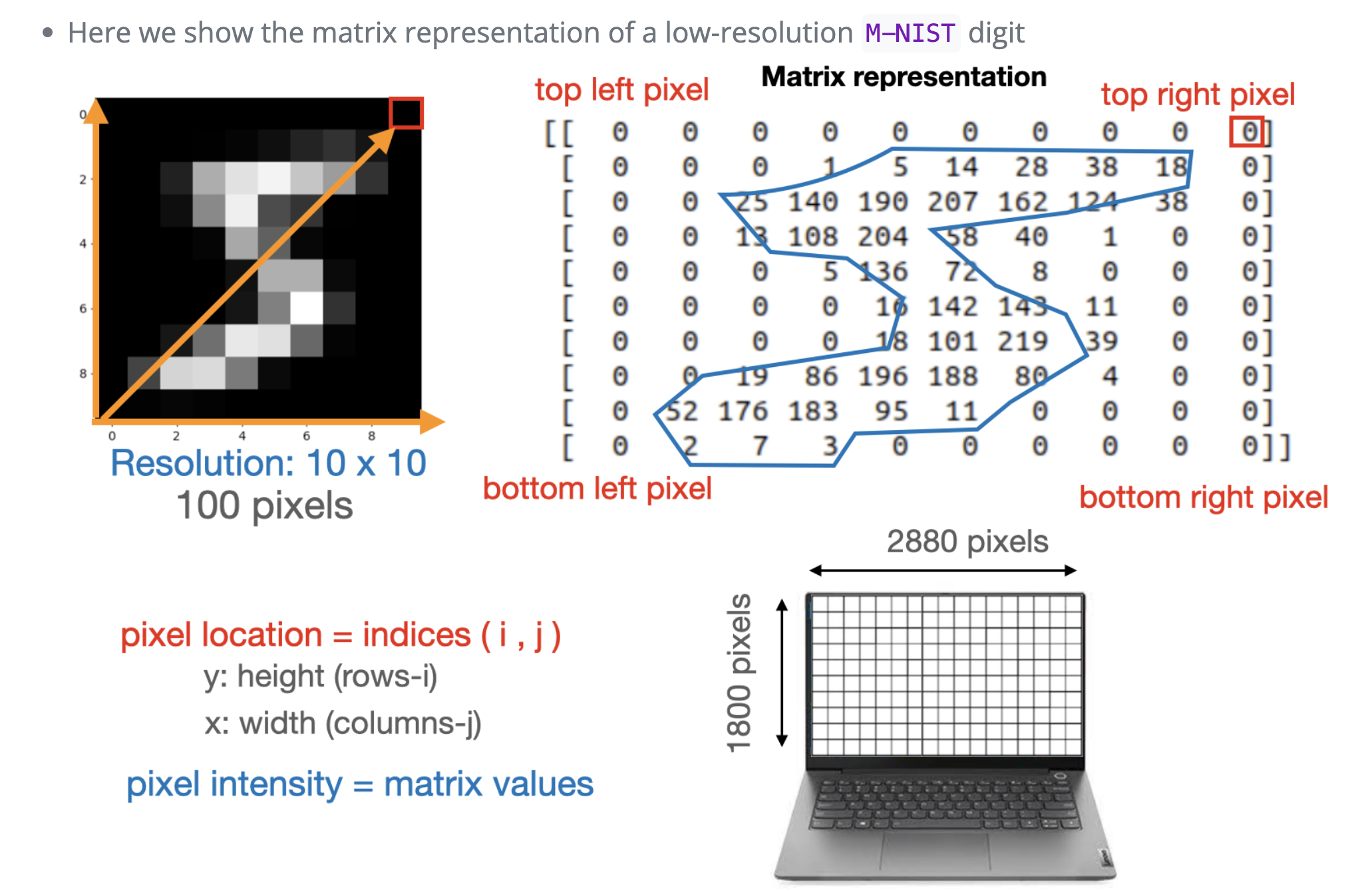
Image data \(\rightarrow\) Computer vision
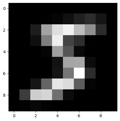
Images become matrices or tensors
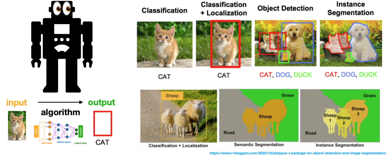
These are the input to the computer’s “eyes”, i.e. computer vision models
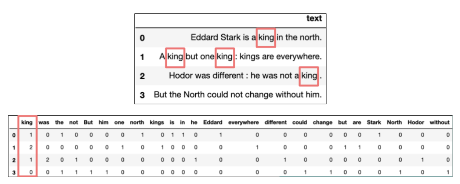
Text data \(\rightarrow\) Natural language processing
Vectorization converts text into a numerical representation that can be used by machine learning models.
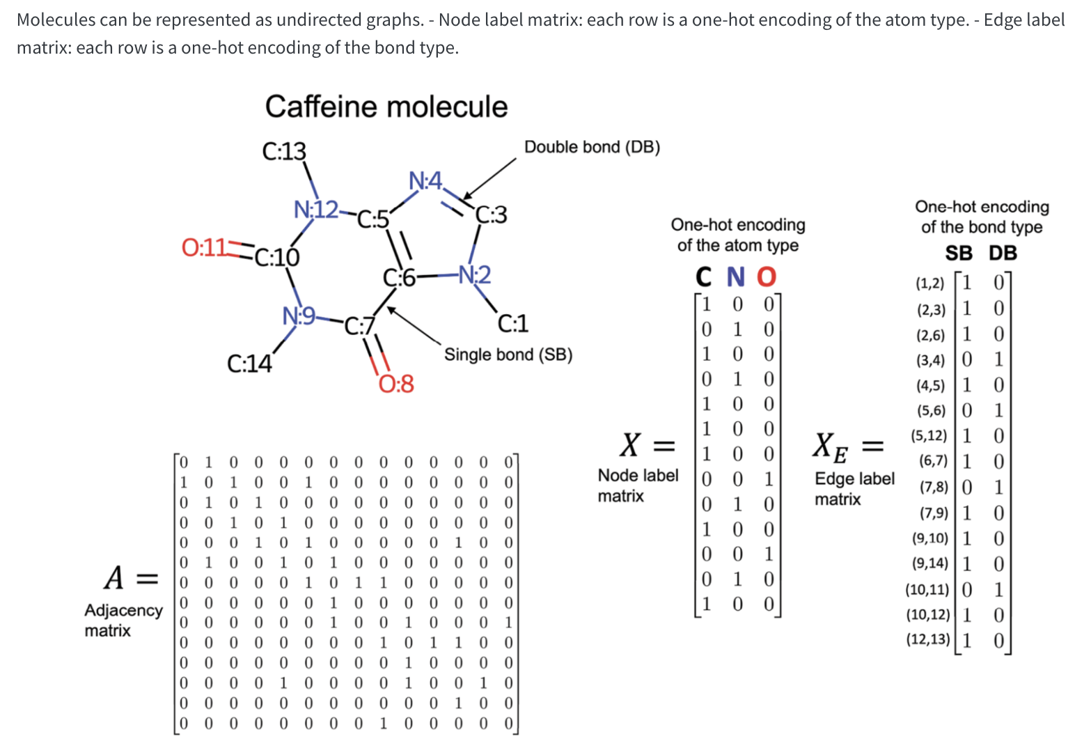
Network data example: Molecular data
`
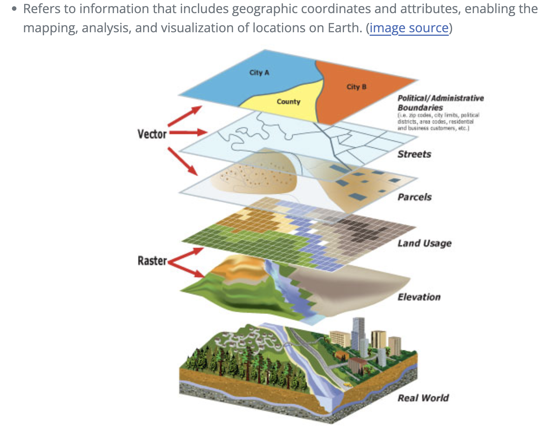
Geo-spatial data
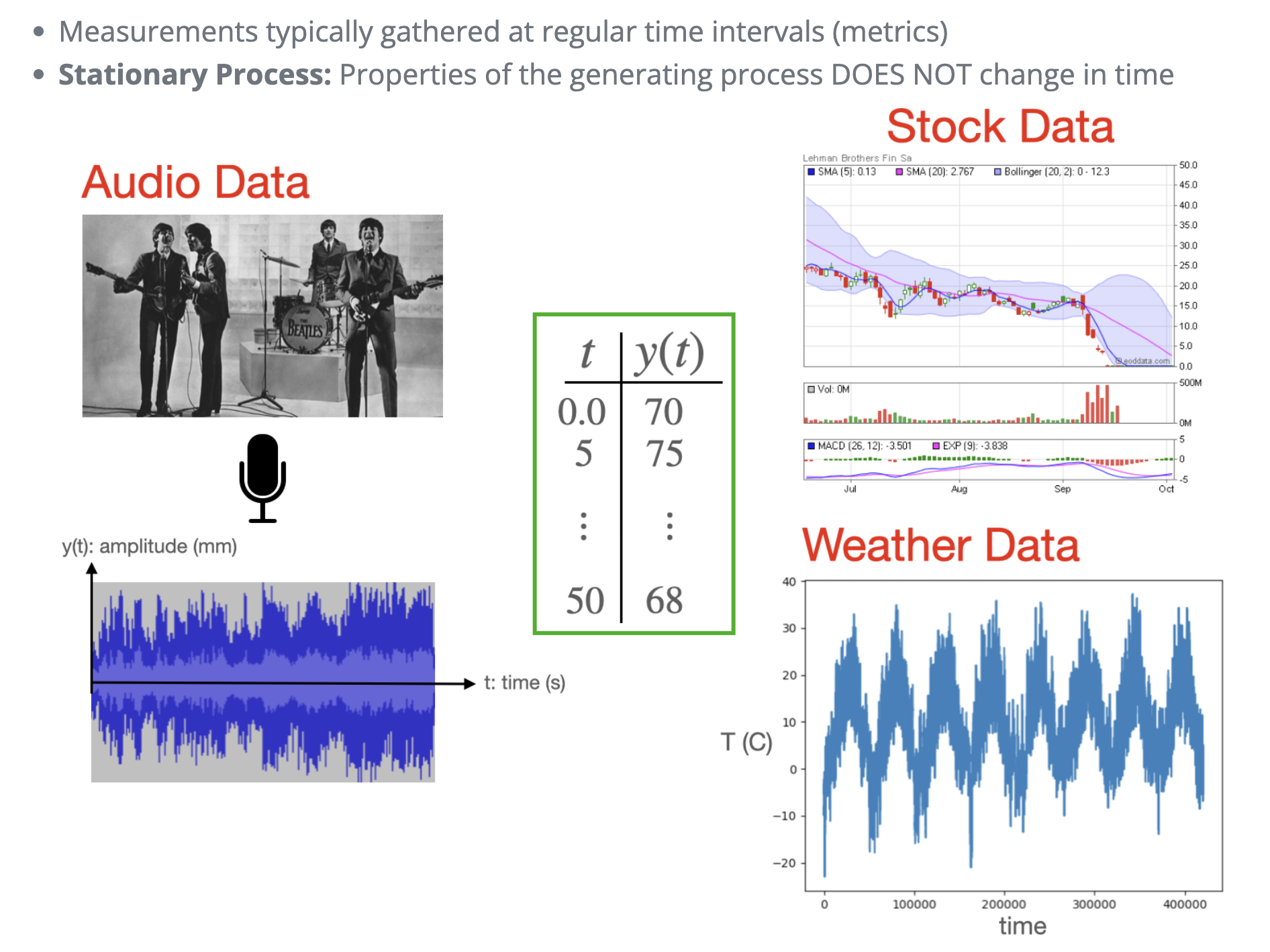
Timeseries
What do we visualize?
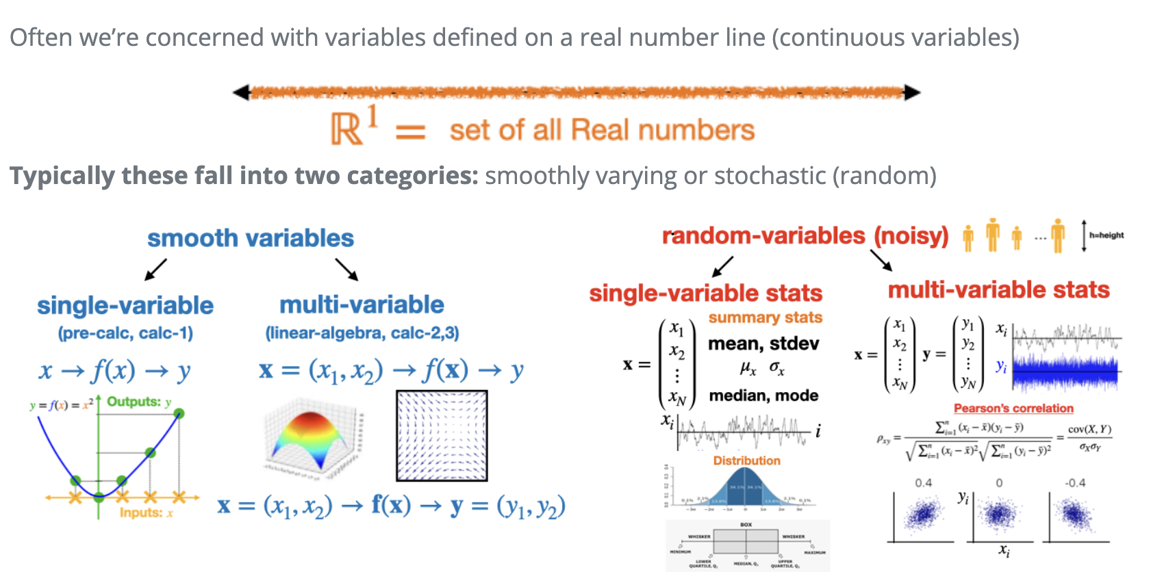
Fundamental entities in visualization
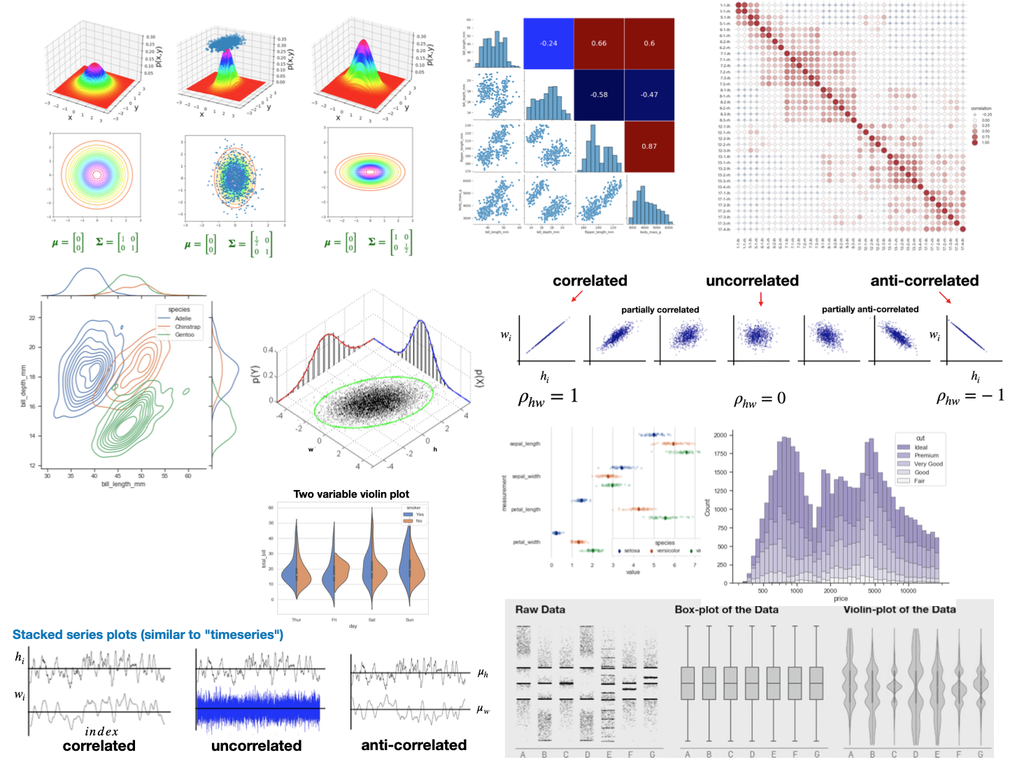
Obviously not all, but most visualizations we will do in this class “boil down” to two broad categories
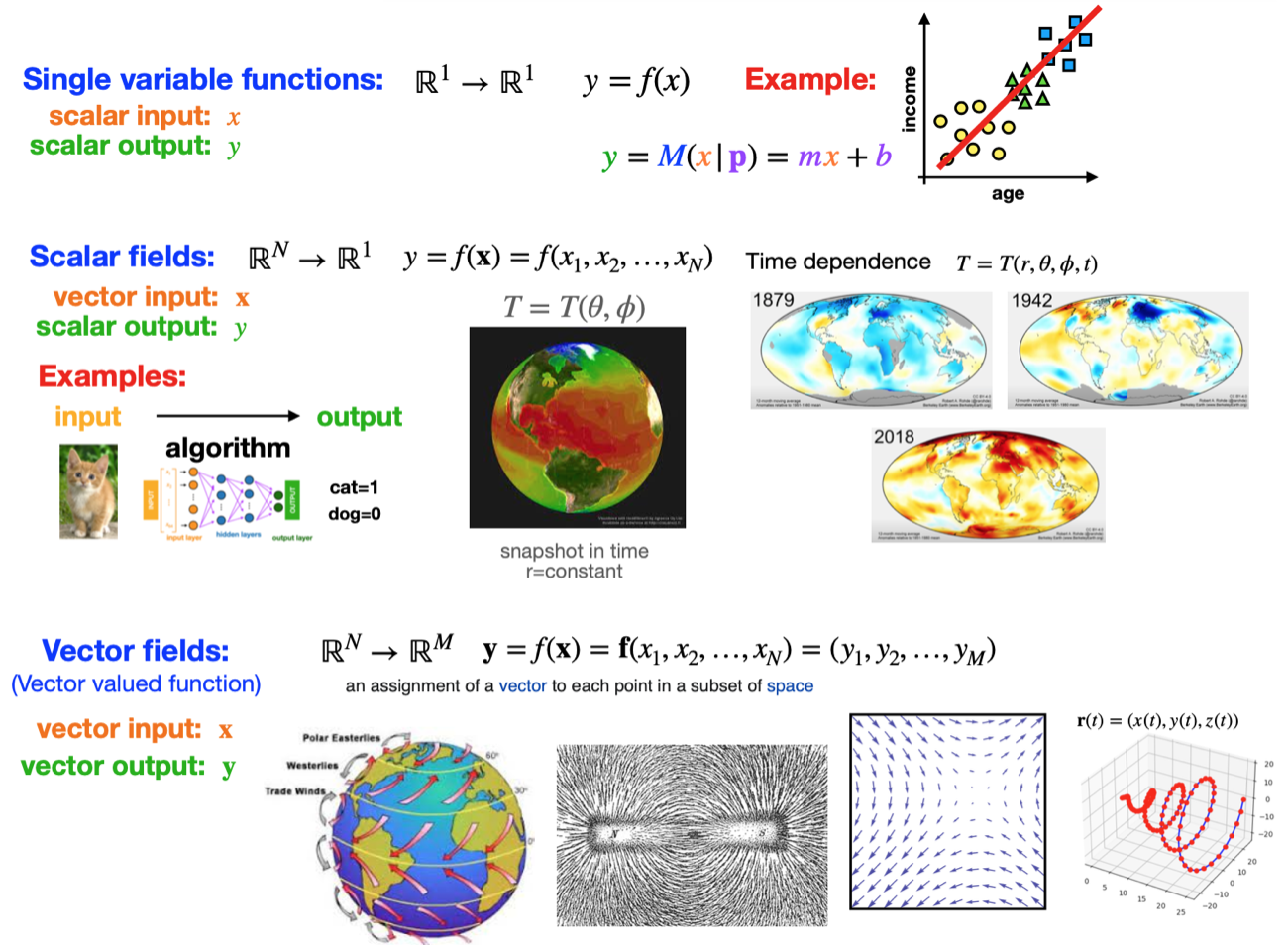
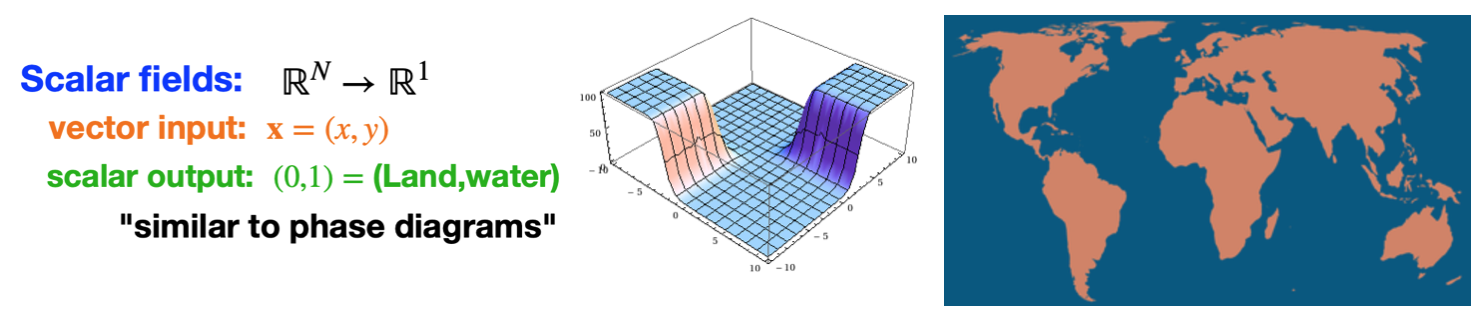
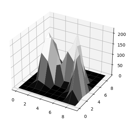
(1): Functions: Either single or multi-variable.
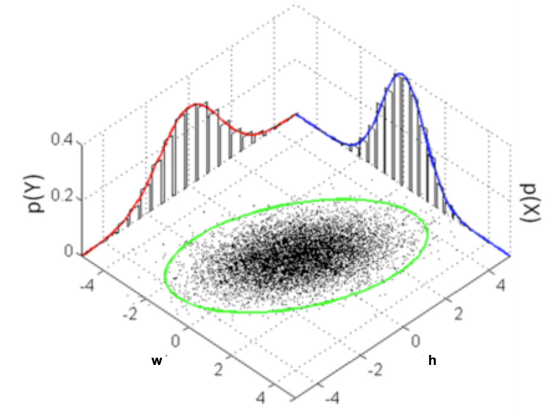
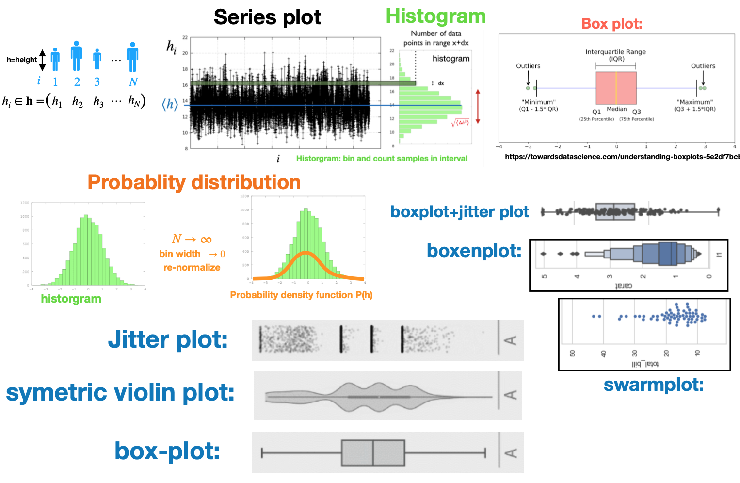
(2): Statistical distributions: Either single or multi-variable.
It is helpful to try to put your data into there “boxes” to know what type of visualization options are available to you
Many of the tools and concepts overlap, however, there are differences
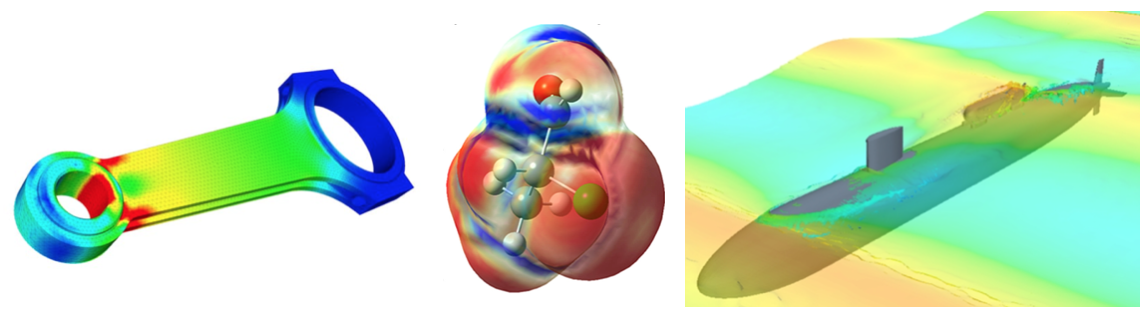
Scientific visualization: The data tends to be “cleaner” and therefore more amenable to certain types of visualizations: smooth surfaces and functions, solutions of differential equations, fluid flux, simulation results, etc
Data visualization: The data tends to be more complicated, statistical, and “messier”. Therefore, different methods are better suited.
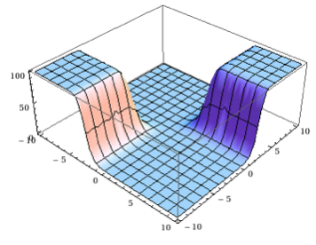
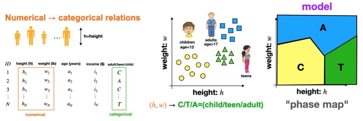
Aside: This type of function is what we try to “learn” in classification tasks
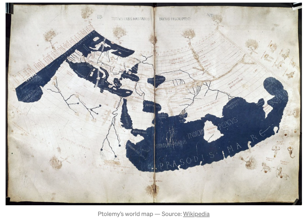
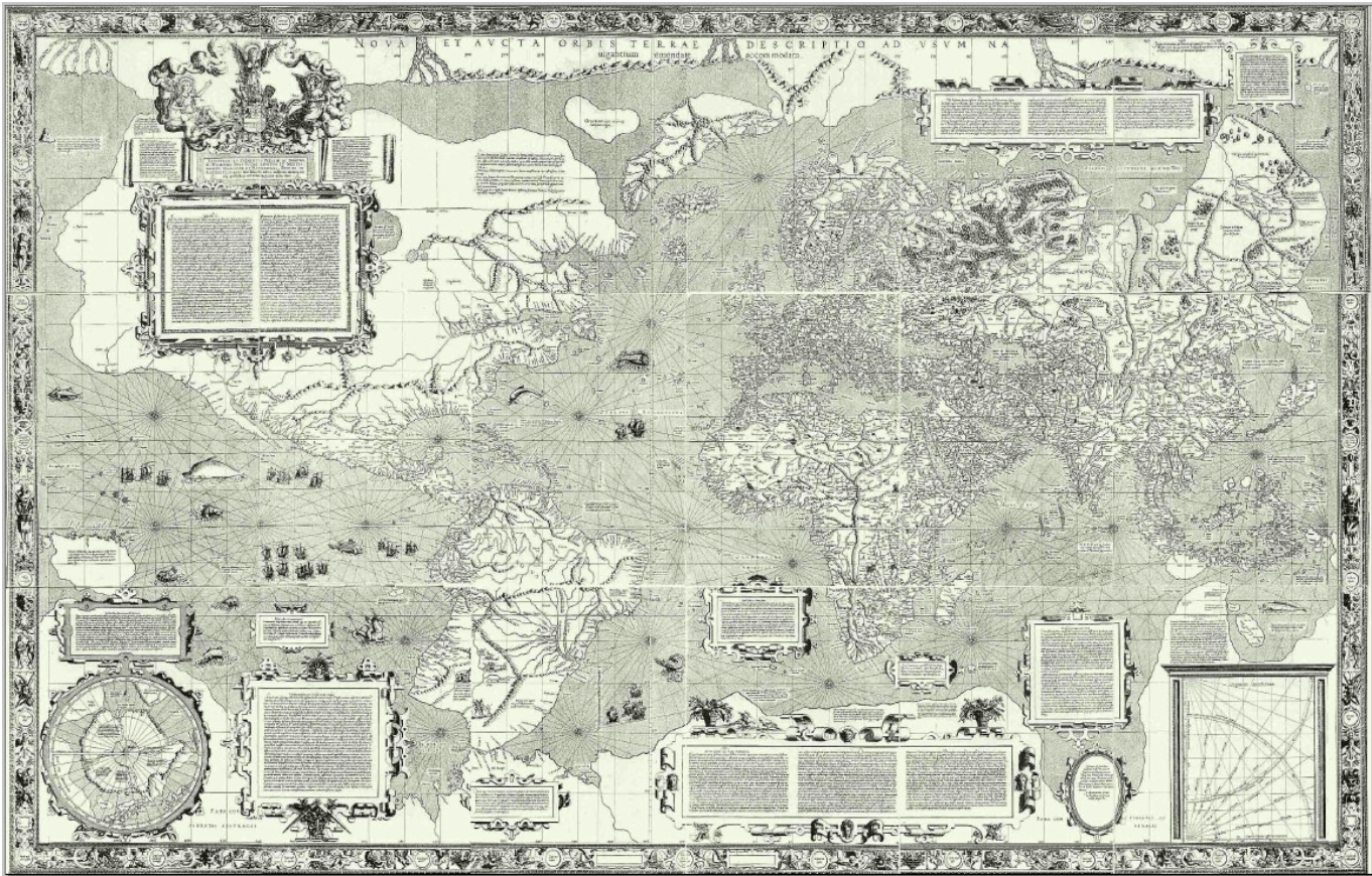
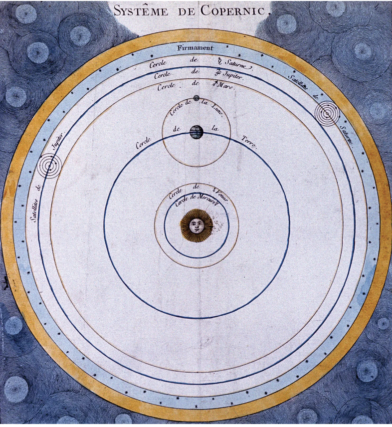
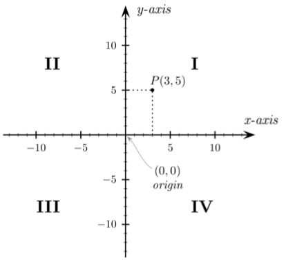
The scientific revolution
Scientific discovery: This was more focused on the mathematics and natural sciences
1543: Nicolaus Copernicus (On the Revolutions of the Heavenly Spheres).
1637: Rene Descartes.
1687: Issac Newton: Mathematical Principles of Natural Philosophy (invented physics)
The industrial revolution-1
Statistics and visualizations made large advances in the mid-19th century
The industrial revolution was the first “data explosion”
Accurate scientific measurements and standards, factory payroll and production data, supply chain and delivery schedules, thermodynamic data from steam engines
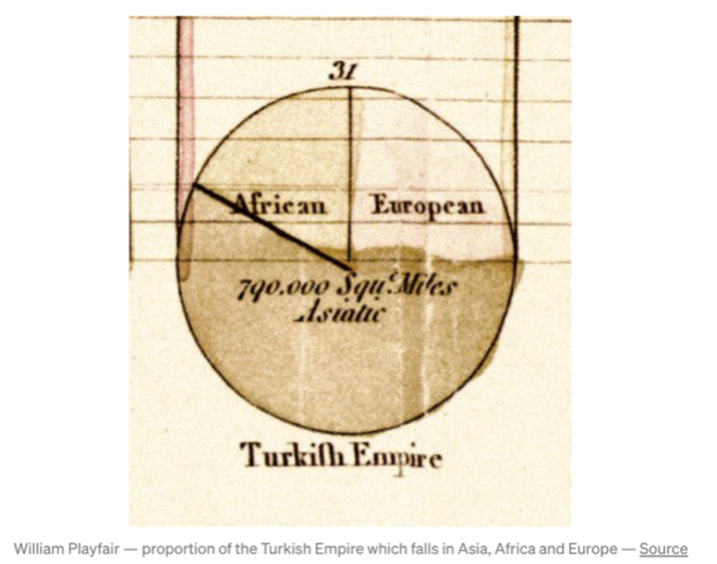
1800-1900: William Playfair Invented the pie chart
The industrial revolution-2
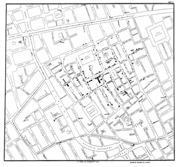
1854: John Snow cholera clusters in London.
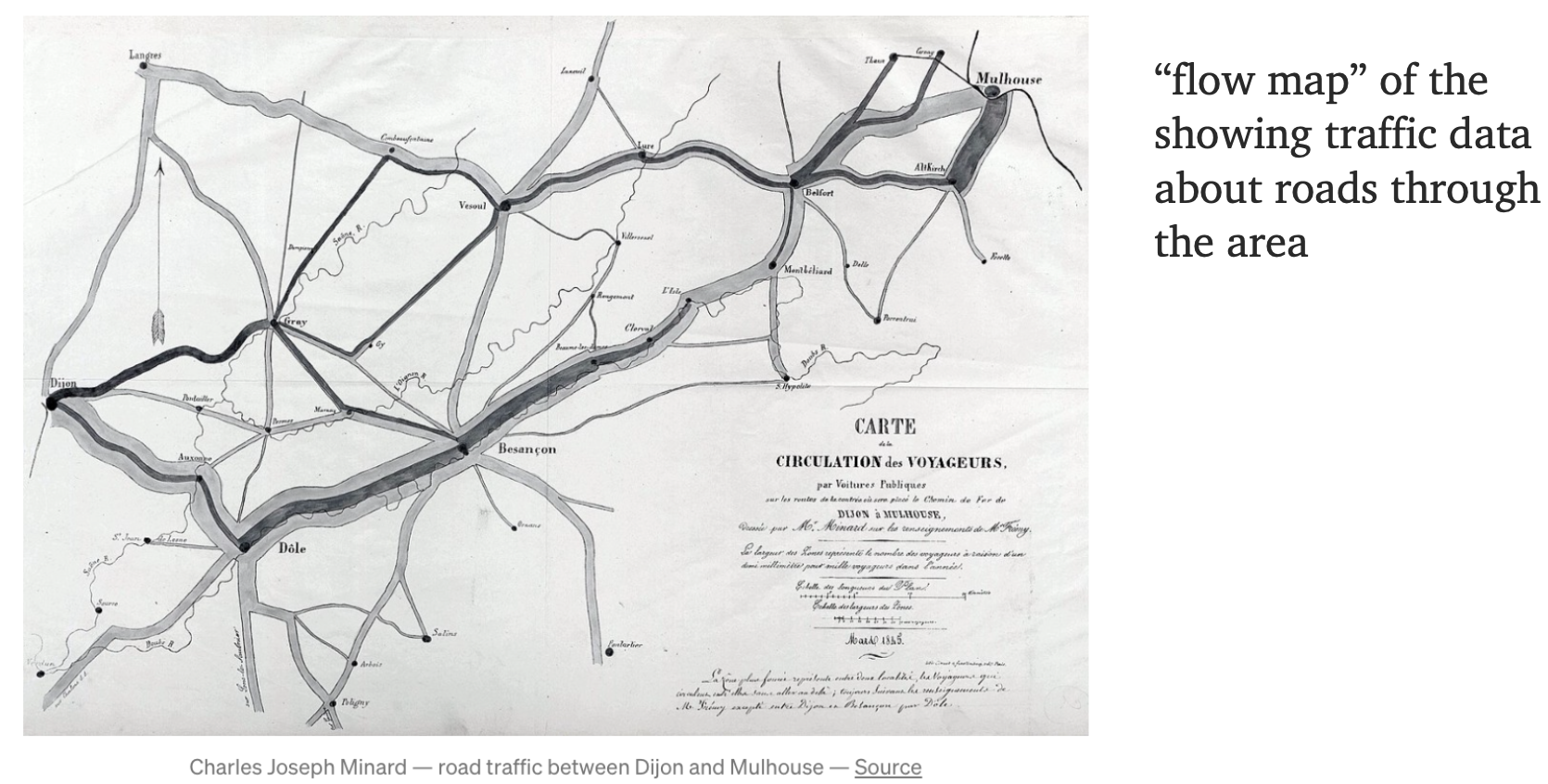
1845: Charles Joseph Minard: Visualizing the flow of people.
The industrial revolution-3
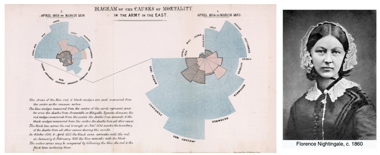
1856: Florence Nightingale: Diagram of the causes of mortality in the army in the East
1913: Iowa State University: Introduced some of the first courses in “graphing” data
The industrial revolution-4
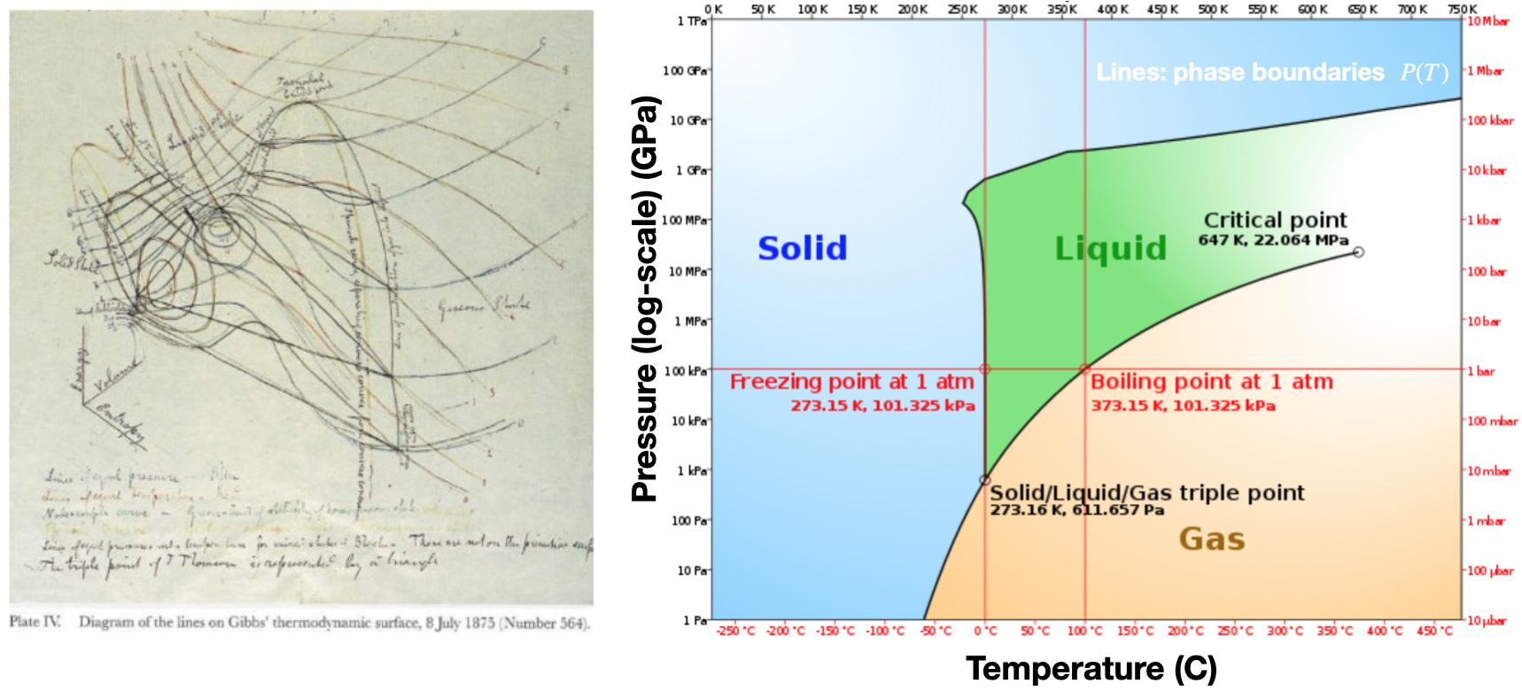
Thermodynamics and chemistry were major accomplishments for early data analysis.
Early pioneers took massive amounts of data (e.g. temperature, pressure, mass, etc), analyzed it, and codified the findings into a well organized and logical theoretical framework (thermodynamics and statistical mechanics)
1875: Josiah Willard Gibbs: Many insights were fueled by creative data visualizations
The information age
1970s: CAD/CAM
1977: Princeton University: Statistics Professor John Tukey Developed the first exploratory data analysis (EDA) using visualizations.
1980s: Scientific and business visualizations (Harvard Graphics)
1983: Edward Tufte published “The Visual Display of Quantitative Information” which showed effective visualization methods.
1990: Excel, Powerpoint, R
1984: Apple Computer introduced the first popular and affordable computer that focused in graphics (GIU) as a mode of interaction and display. This was huge and persists today. (Modified from version at IMB)
1999: The words, “information visualization” were so first named in the book: “Readings in Information Visualization: Using Vision to Think”, Card, Mackinlay, Shneiderman
Data visualization is now so ubiquitous that it’s hard to imagine a time without it
Importance of data visualization
Data visualization is more important than ever!
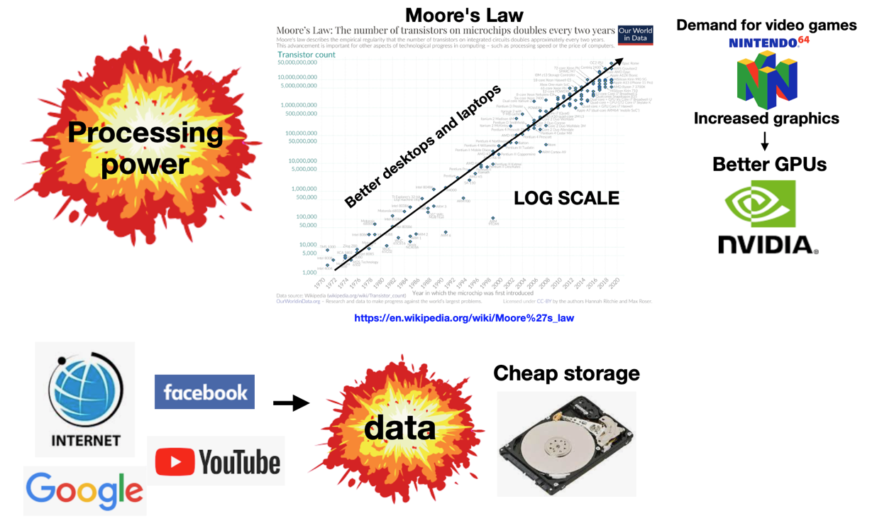
The amount of data in the “information age” dwarfs that of previous eras.
Tool stack: Big picture overview
Core Technologies for Data Visualization
Markdown: Lightweight language for formatting notes, documentation, and slides.
Jupyter Notebooks: Interactive computational documents combining code, visualizations, and narrative.
RMarkdown or Quarto: Tools for combining code, text, and visualizations in a single document.
Python: Widely used programming language with a strong data science and plotting ecosystem (e.g., matplotlib, seaborn, pandas).
R: Statistical programming language with powerful data visualization packages (e.g., ggplot2).
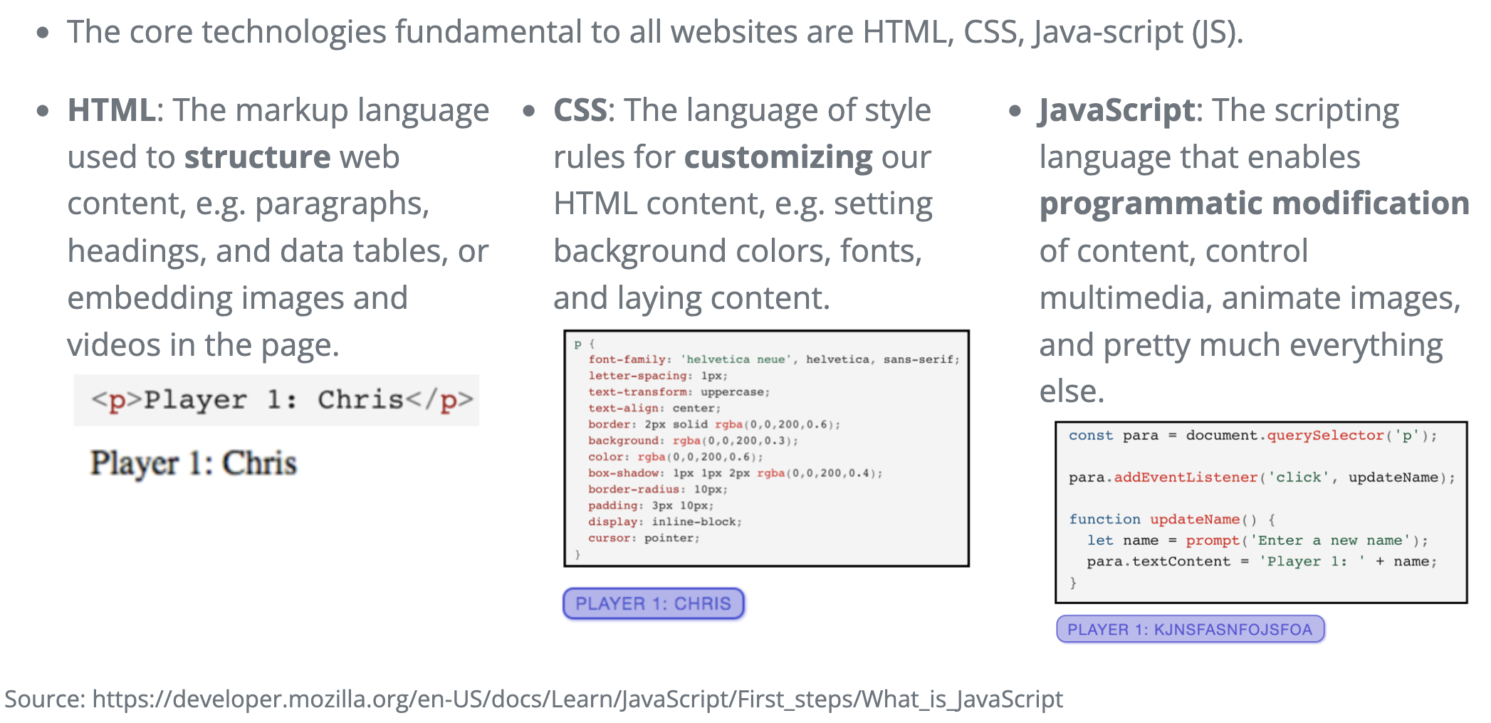
HTML, CSS, JavaScript: The foundation of most web-based visualizations (e.g., D3.js, Plotly.js, Quarto publishing).
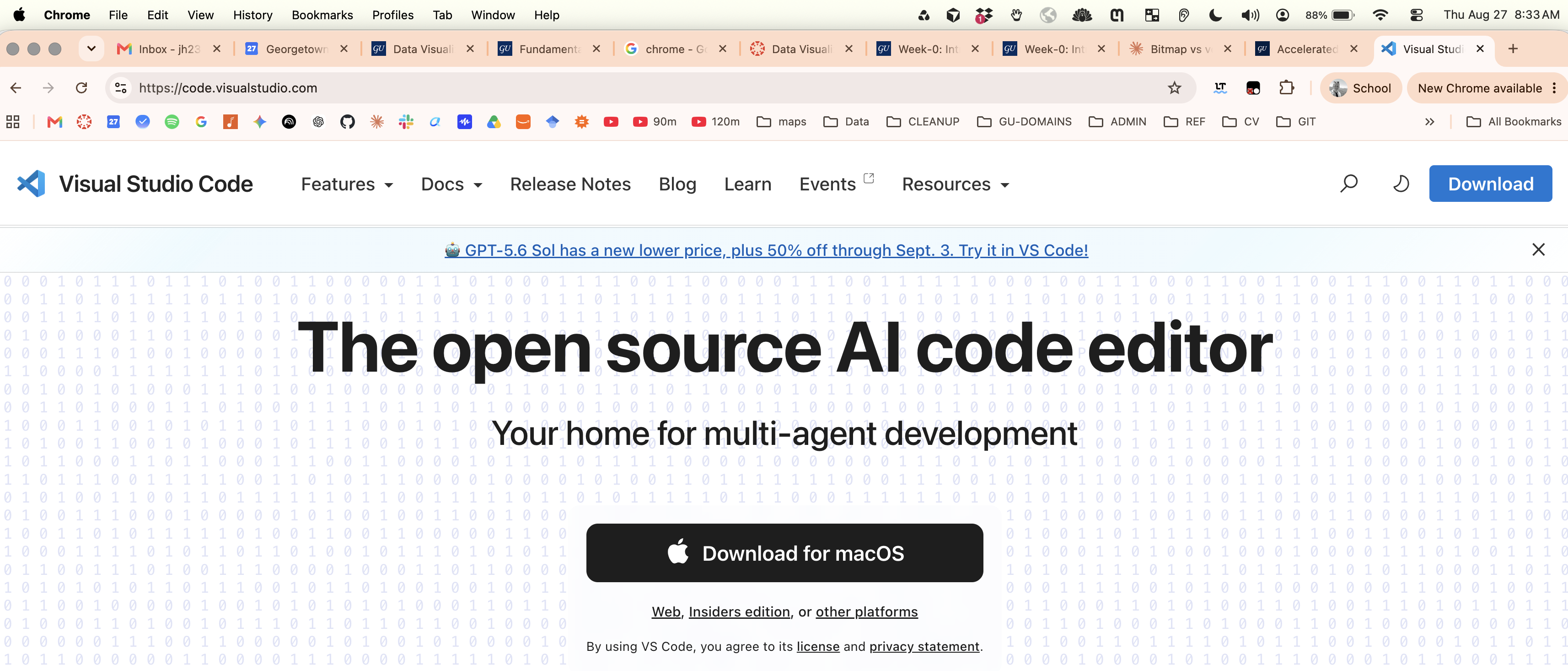
VS Code: Popular code editor/IDE for writing and running code, managing notebooks, and integrating with many languages.
Git: Version control system for tracking changes in any set of files.
GitHub: Web-based hosting service for version control using Git.
VS code:
This is the code editor that I will primarily be using throughout the course.
It’s arguably the most popular code editor or integrated development environment (IDE) in the world. And I would recommend it over something like a language specific IDE such as R Studio.
Web publishing: HTML, CSS, and JavaScript
This is NOT a web development class, but it is important to understand the basics of how the web works, since most visualization libraries are built on these technologies.
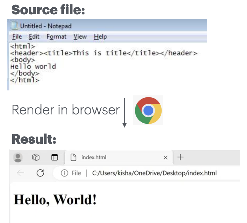
HTML: Hello world
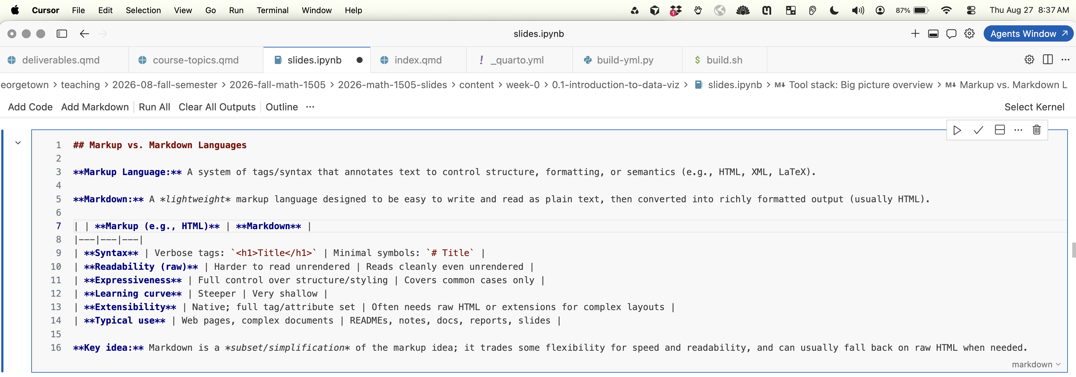
Markup vs. Markdown Languages
Markup Language: A system of tags/syntax that annotates text to control structure, formatting, or semantics (e.g., HTML, XML, LaTeX).
Markdown: A lightweight markup language designed to be easy to write and read as plain text, then converted into richly formatted output (usually HTML).
Markup (e.g., HTML)
Markdown
Syntax
Verbose tags: <h1>Title</h1>
Minimal symbols: # Title
Readability (raw)
Harder to read unrendered
Reads cleanly even unrendered
Expressiveness
Full control over structure/styling
Covers common cases only
Learning curve
Steeper
Very shallow
Extensibility
Native; full tag/attribute set
Often needs raw HTML or extensions for complex layouts
Typical use
Web pages, complex documents
READMEs, notes, docs, reports, slides
Key idea: Markdown is a subset/simplification of the markup idea; it trades some flexibility for speed and readability, and can usually fall back on raw HTML when needed.
Markdown: hello world
Markdown editor
There are many markdown editors.
It’s good to have one installed on your computer. You can use whichever one you are most comfortable with.
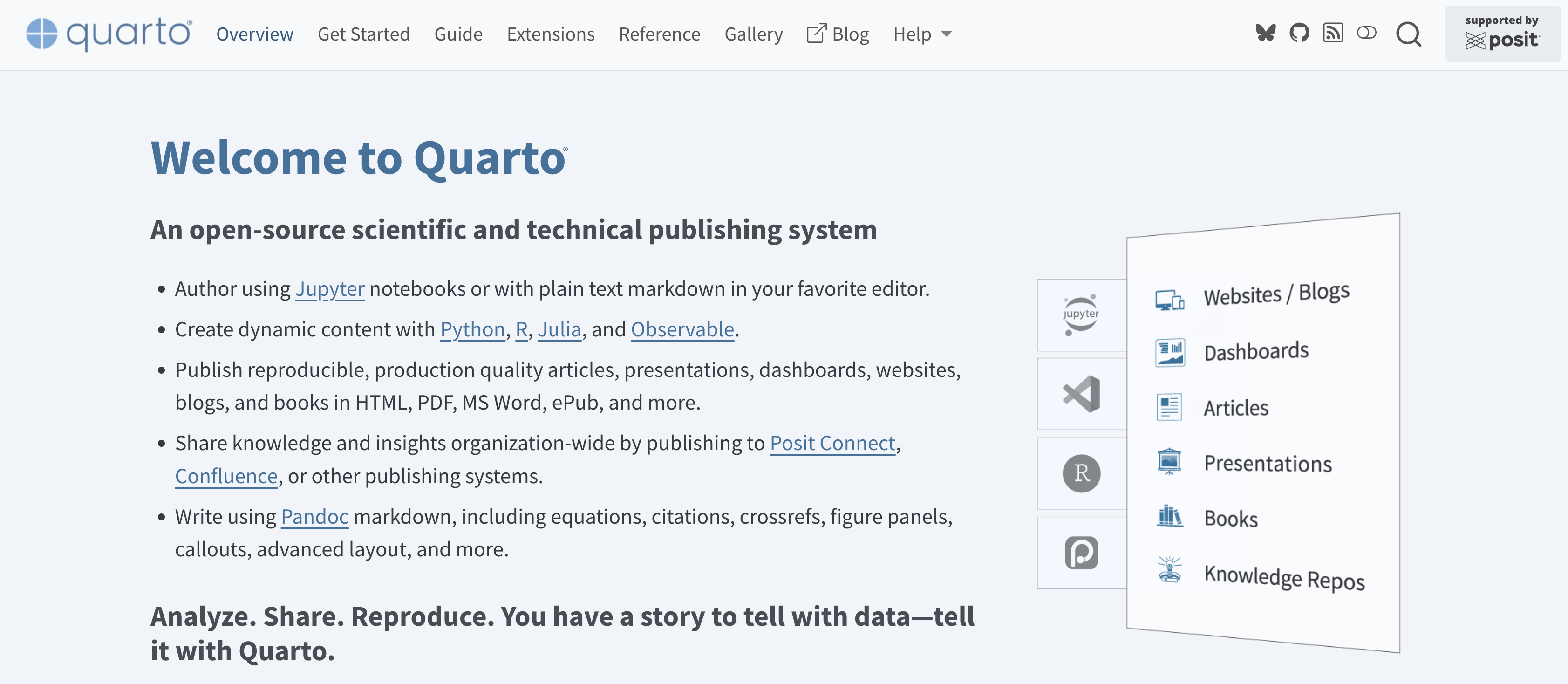
An open-source scientific and technical publishing system for creating dynamic, reproducible documents from code.
Multi-language: Works with Python, R, Julia, and Observable JS, often in the same document
Literate programming: Combine narrative text, code, and output (plots, tables, results) in one source file
One source, many outputs: Render the same .qmd file to HTML, PDF, Word, slides (reveal.js), websites, and books
Built on Pandoc: Inherits robust Markdown-based formatting and citation support
IDE-agnostic: Works in VS Code, RStudio, Jupyter, or the command line
Successor to R Markdown: Generalizes the same idea beyond R to a language-agnostic tool
Why it matters here: Quarto lets you build reproducible reports and slide decks where the code, visualization, and write-up all live together and stay in sync.
More on this later in the course …
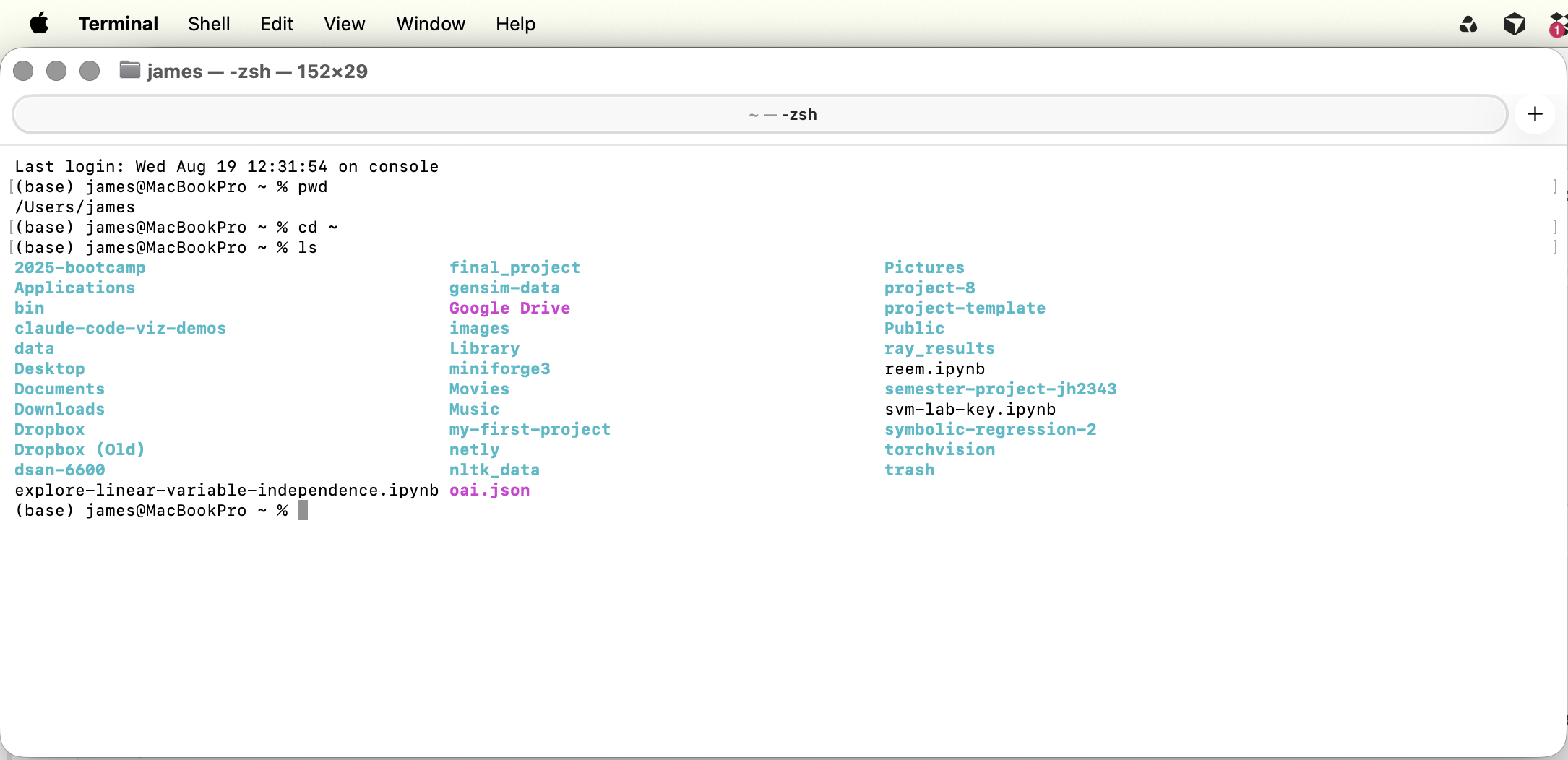
Command line interface: CLI
This is not a main focus of the class, but I highly recommend you embrace it as a fundamental way to interact with your computer.
Another reason to learn: Modern Agentic Ai tools are largely CLI-based (e.g. Claude-Code)
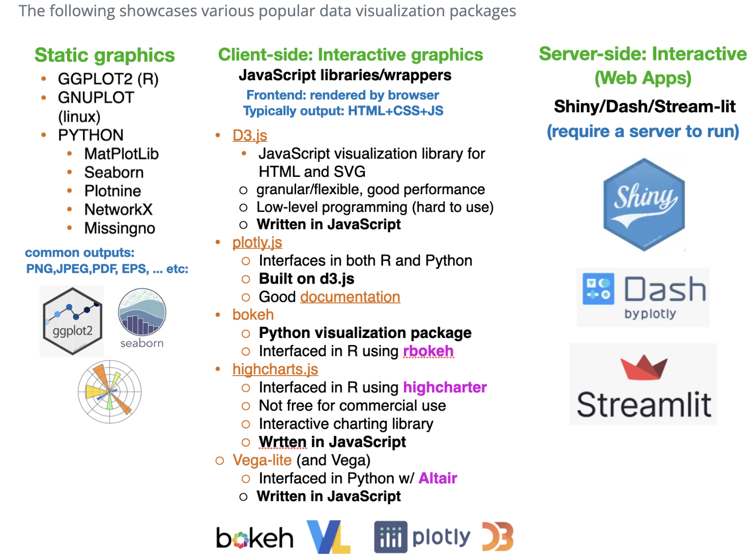
Popular data-vis packages
Graphical formats
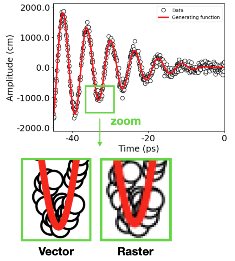
Vector vs raster (i.e. bitmap) graphics
Overview: Bitmap vs. Vector Graphics
Two fundamentally different ways to represent an image on a computer.
Bitmap (Raster) Graphics: An image made of a fixed grid of pixels, where each pixel is assigned a specific color. The image is essentially a big table of color values.
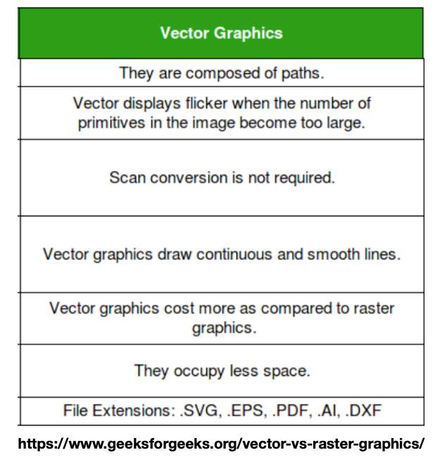
Vector Graphics: An image made of mathematical descriptions; points, paths, curves, and fills; that a computer calculates and draws on demand.
Bitmap / Raster
Vector
What it stores
A grid of pixels, each with a color value
Mathematical shapes: points, lines, curves, fills
Scaling
Blurs / pixelates when enlarged
Scales to any size with no loss of quality
Best for
Photographs, detailed / continuous-tone images
Logos, icons, diagrams, type, charts
File size
Grows with resolution & dimensions
Grows with number of shapes, not resolution
Resolution
Fixed; tied to pixel count (DPI/PPI)
Resolution-independent
Editing
Edit pixels; hard to isolate objects
Edit individual objects & their properties
Common formats
PNG, JPEG, GIF, BMP, TIFF
SVG, PDF, EPS, AI
Takeaway: Raster describes what each dot looks like; vector describes how to draw the shapes. The right choice depends on the content and how the image will be used.
Vector graphics
Vector graphics are more like a coding language which makes them easy to change programmatically
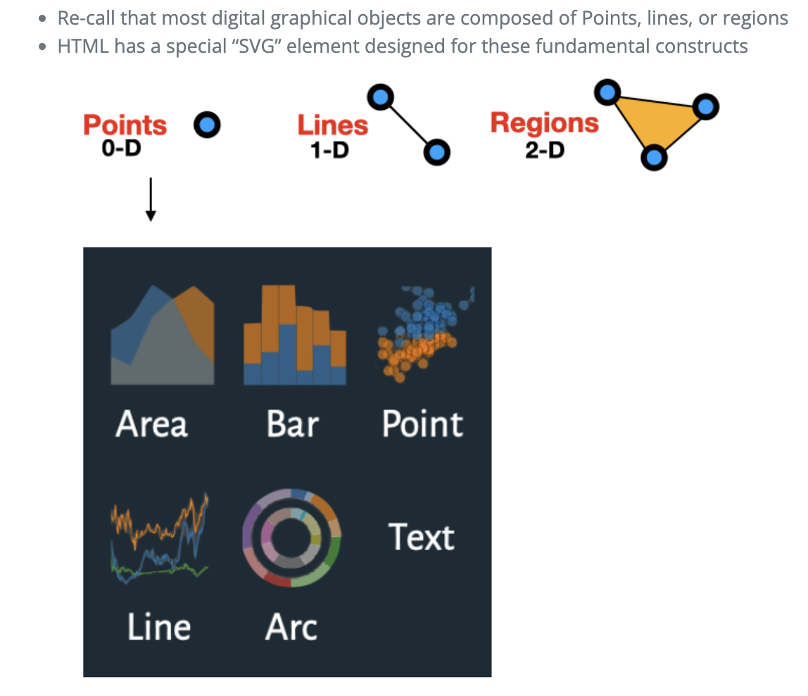
Building blocks of graphics
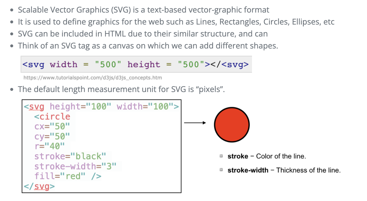
SVG elements
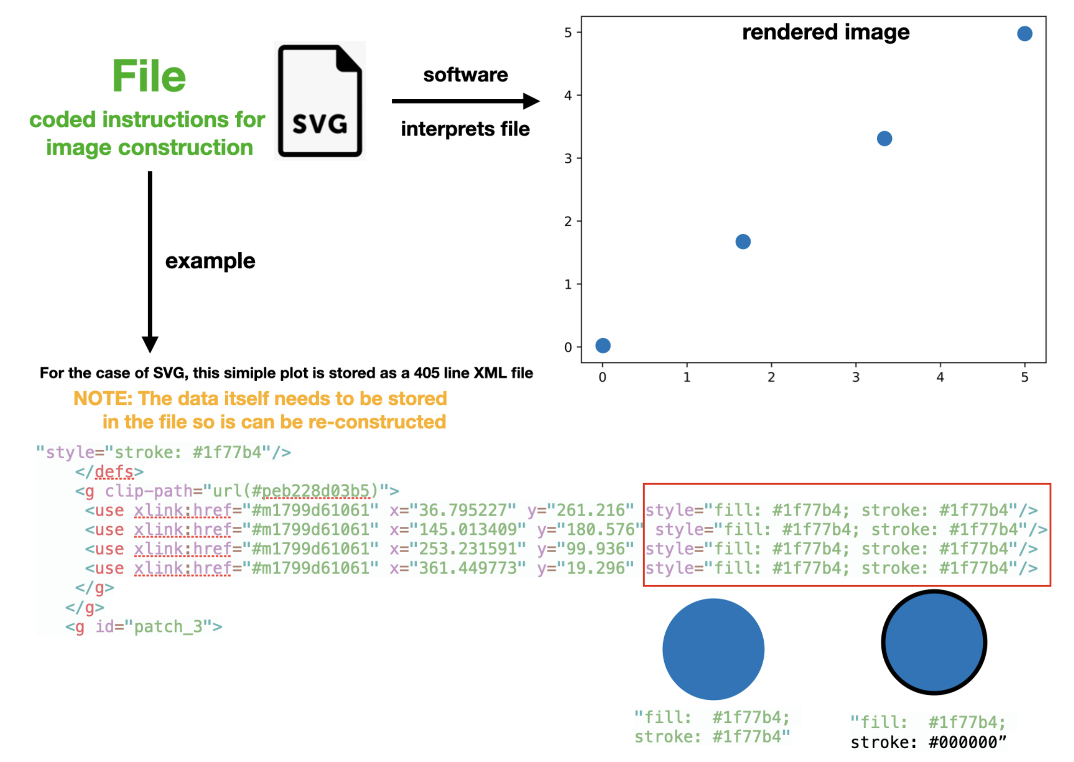
Vector graphics example: SVG
Vector graphics are more like a coding language which makes them easy to change programmatically
Example
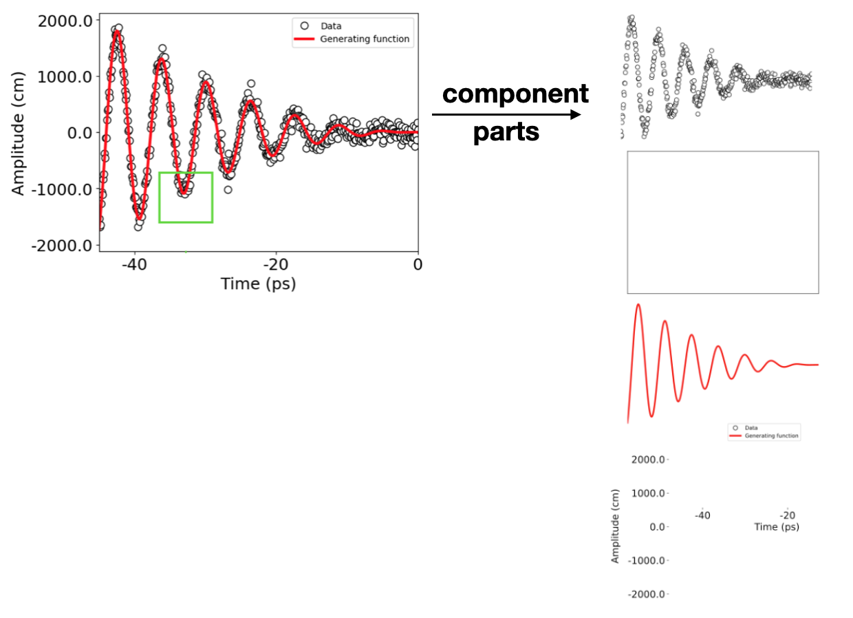
Vector graphics are composed of a layered structure with groups of objects
Think of them like a blank canvas with elements and groups added on top
Vector graphics: Pros
Can change them programmatically (which facilitates interactivity)
Easier to edit (change colors of lines, change fonts, move points, etc)
Image can re-render to increase resolution when zooming in (can rescale to any size).
Raster graphics (Bitmaps)
Motivation
Why should you care about how computers store images and graphics?
It will help you better understand and manipulate the visualizations you generate in ANLY-503
Images are data!! Understanding image data is the first step in understanding computer vision and other advanced applications
Types of digital images
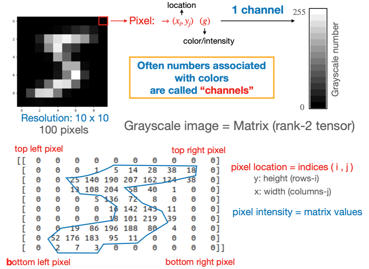
Raster graphics: A raster graphic represents a two-dimensional picture as a matrix of pixels (bitmap)
this matrix can be rendered via a computer display. 1
In this context, the images are stored as matrices
Examples: .PNG, .BMP, .TIF, .GIF, .JPG
Vector graphics: Visual images are created directly from geometric shapes defined on a Cartesian plane, such as points, lines, curves and polygons. 2
In this context, images are stored as a set of coded instructions, similar to HTML
The images can be “re-constructed” and “rendered” using specialized software to parse these instructions into images
Examples: .SVG, .EPS, .PDF, .AI, .DXF, .HTML
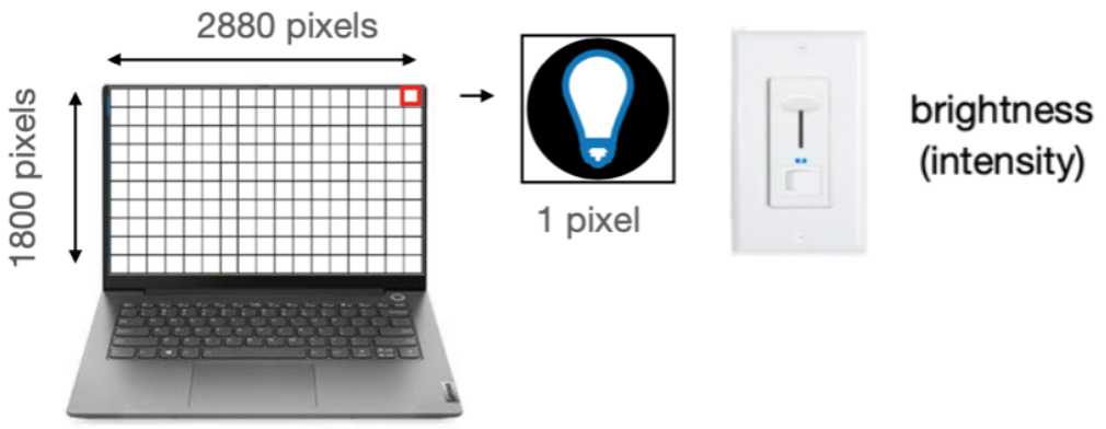
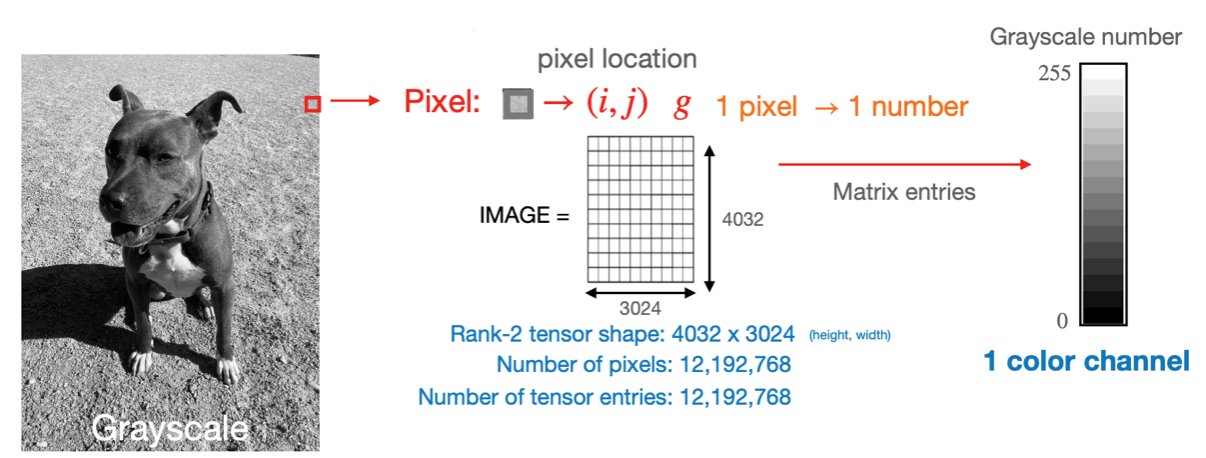
Black and white screens
Understanding some basic concepts about screens is useful
In a black and white screen the pixels are variable light bulbs outputting white light
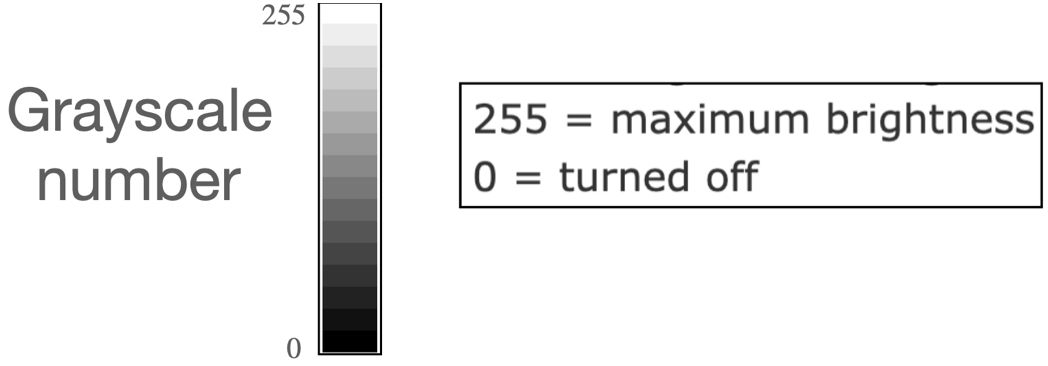
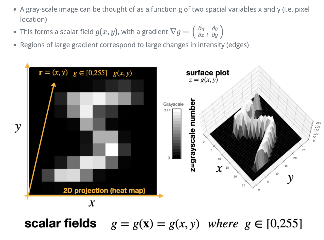
The intensity of a pixel’s light is control by the gray-scale number.
Grayscale images
Black and white images are stored by specifying the gray-scale number for all the pixels
The pixel location is determined by its location in the matrix.
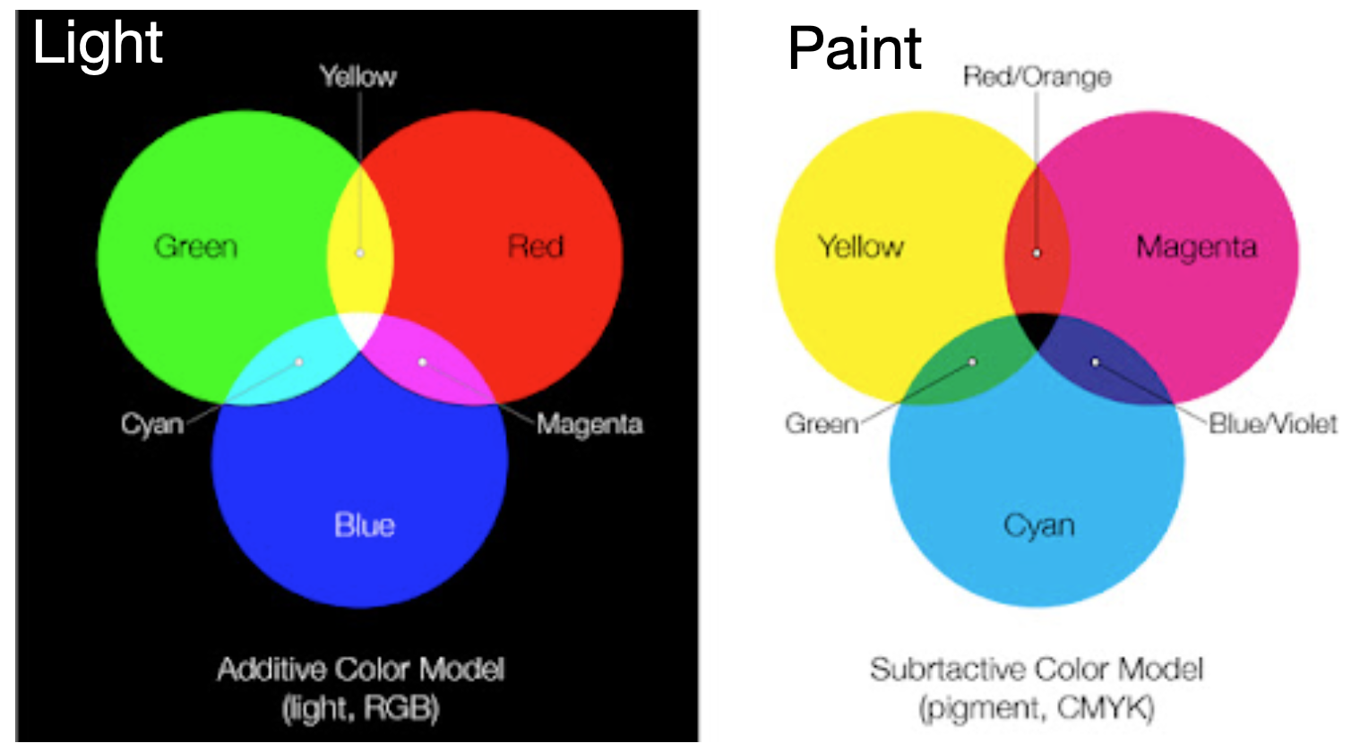
Color mixing
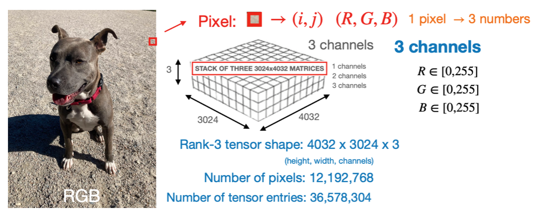
Color pixels
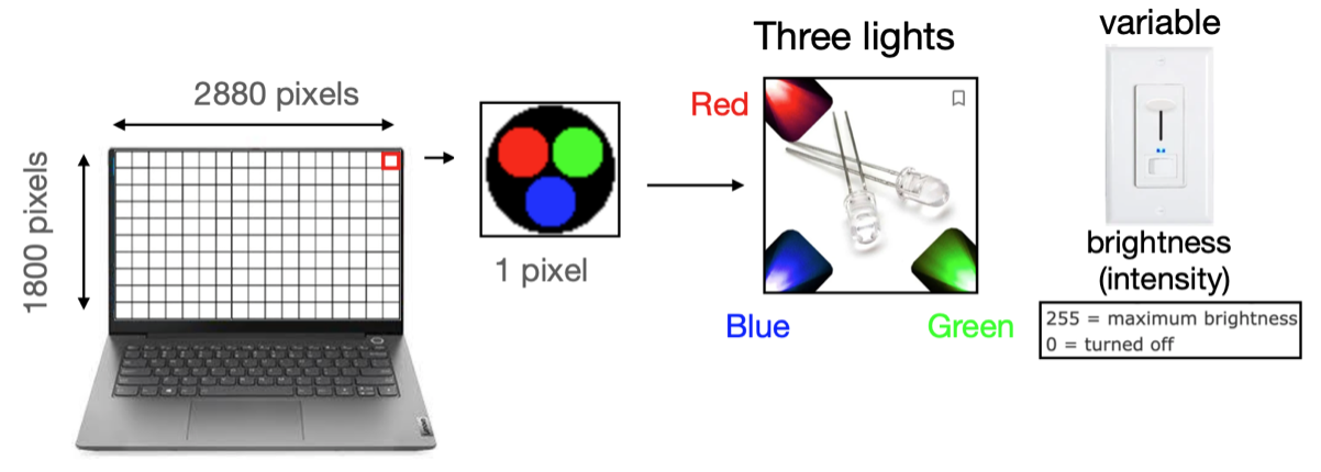
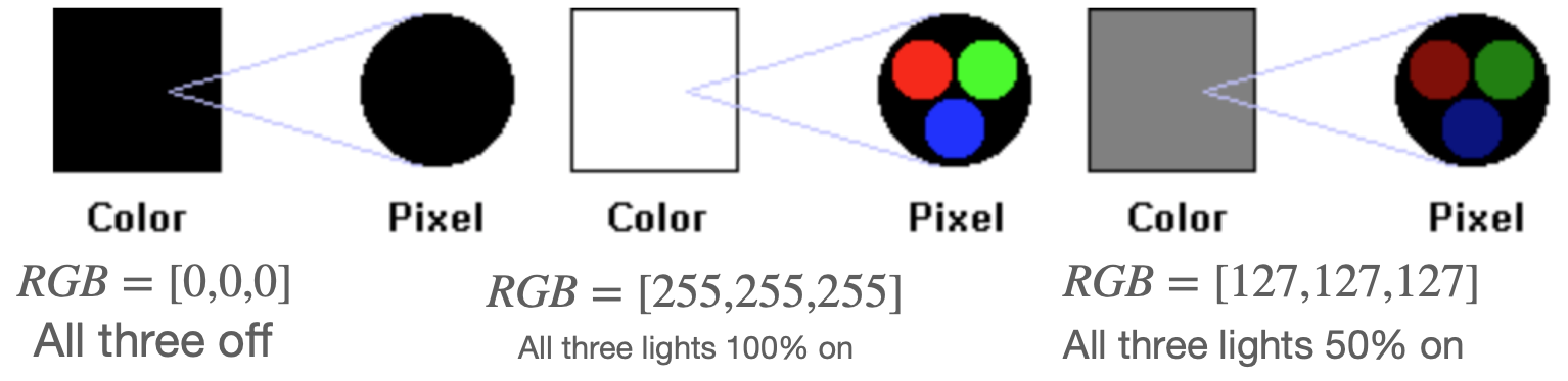
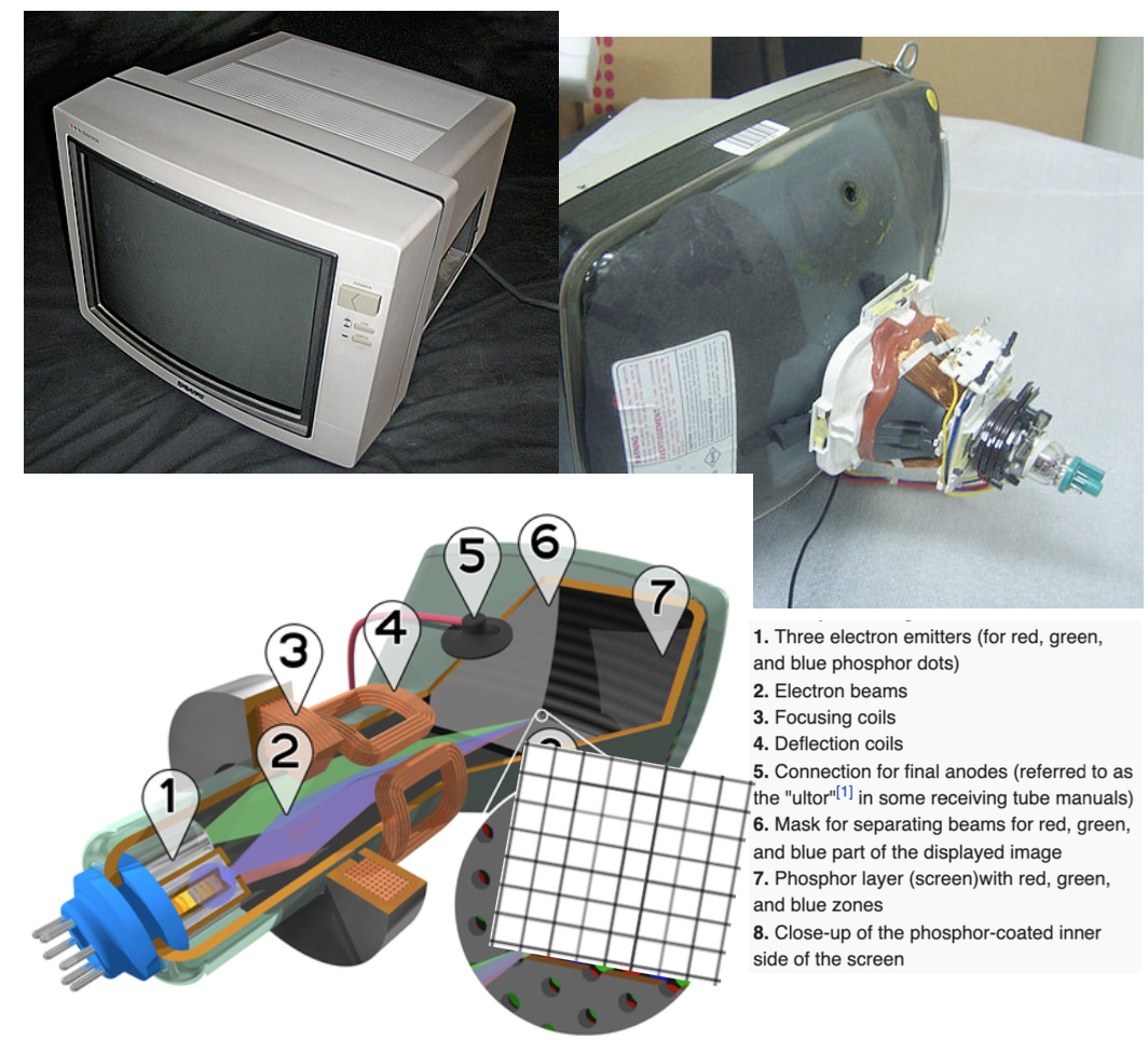
In a color screen the pixels are variable light bulbs outputting red, green, or blue light.
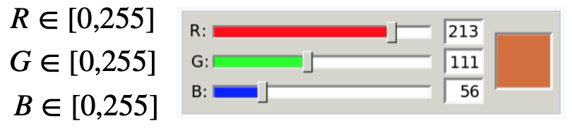
We need three numbers (R,G,B) for each pixel to control the brightness of the 3 lights
These three numbers allow us to form different colors through color-mixing
There are \(255 \times 255 \times 255 = 16,581,375\) possible colors on the computer screen
Color examples-1
Gray-scale is achieved by turning all three lights on at equal intensities \(R=G=B\)
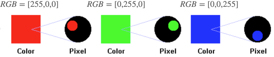
Primary colors: One light on at a time Image source: https://www.chem.purdue.edu/gchelp/cchem/RGBColors/body_rgbcolors.html
Color examples-2
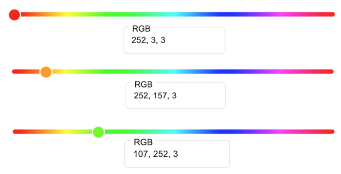
Secondary colors: Two lights on at a time with equal intensities
General colors: Three lights on at a time with different intensities Image source: https://www.chem.purdue.edu/gchelp/cchem/RGBColors/body_rgbcolors.html
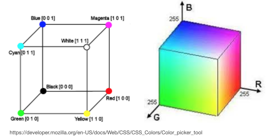
RGB Color cube
Grayscale \(\rightarrow\) main diagonal (R=G=B)
Secondary \(\rightarrow\) two lights on at full intensity (outer surface)
mixed \(\rightarrow\) three lights w/ different intensity (cube interior).
Mathematical description
Grayscale: matrices (e.g. np.shape=(320,120) or np.shape=(320,120,1)).
RGB: Rank-3 tensors (stack of matrices)(e.g. np.shape=(320,120,3)).
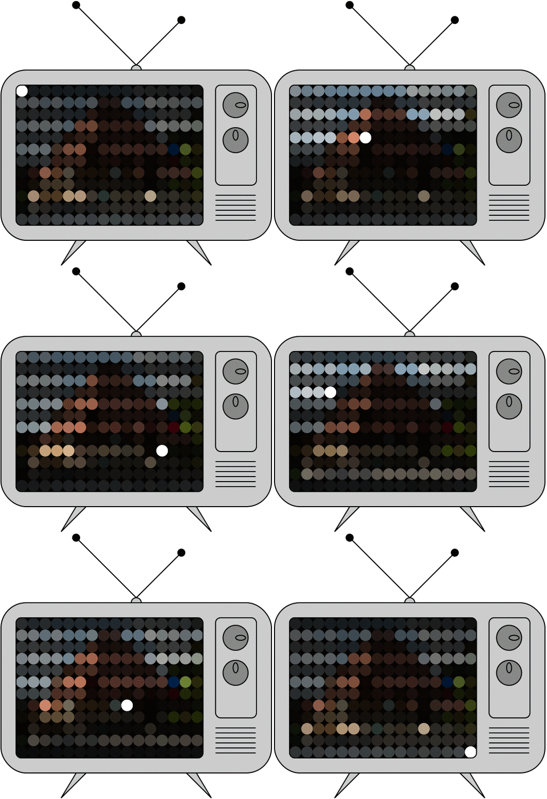
Image rendering
Images show up on the screen by rastering accross the matrix and lighting up the relevant pixels one by one
Human eye can see roughly 30-60 frames per second
Refresh rate Is the number of times per second the display draws a new image.
Pros: Simple and intuitive, highly mathematical, well suited for computer vision applications, can manipulate manually in Power-point or photo-shop (run demo)
Cons:
Hard to manipulate programmatically, so no interactive raster graphics
Harder to change once rendered
Larger matrices –> higher resolution –> more space on disk
Finite resolution: Image resolution is FIXED and controlled by the matrix size