Univariate and Multivariable Statistics Fundamentals
Recording-1: Univariate (one variable)
Recording-2: Bivariate (two variables)
Part 1: Univariate (one variable)
Setup. You work at a tree farm and measure the height of six red oak trees that were all planted in the same year (20 years ago). Growth tables list red oaks of this age at roughly 31 to 39 ft. Assume height in the population is normally distributed with population mean \(\mu = 35\) ft and standard deviation \(\sigma = 4\) ft.
Normal PDF. \(f(x) = \dfrac{1}{4\sqrt{2\pi}}\exp\!\left(-\dfrac{(x-35)^2}{32}\right)\)
| \(i\) | 1 | 2 | 3 | 4 | 5 | 6 |
|---|---|---|---|---|---|---|
| Height \(x_i\) (ft) | 35 | 30 | 39 | 32 | 36 | 32 |
1.1 Measures of Center
(a) Compute the sample mean \(\bar{x}\).
Answer.
\[ \begin{aligned} \bar{x} &= \frac{1}{N}\sum_{i=1}^{N} x_i = \frac{1}{6}\left(35 + 30 + 39 + 32 + 36 + 32\right) \\ &= \frac{204}{6} \\ &= 34 \text{ ft} \end{aligned} \]
(b) Write the sorted data and compute the median.
Answer.
Sorted: \(30,\ 32,\ 32,\ 35,\ 36,\ 39\)
\(N = 6\) is even, so average the 3rd and 4th values:
\[ \text{median} = \frac{32 + 35}{2} = \frac{67}{2} = 33.5 \text{ ft} \]
(c) Are the mean and median measures of center or spread?
Answer. Both are measures of center.
(d) In one sentence, why is \(\bar{x}\) close to, but not equal to, \(\mu = 35\)?
Answer. Our six trees are one small random sample from the population, so \(\bar{x}\) fluctuates around \(\mu\) from sample to sample (sampling variability) and will rarely land exactly on it.
1.2 Deviations
\(d_i = x_i - \bar{x}\). Fill in the \(d_i\) column (the other columns are for 1.3 and 1.4).
Answer. Using \(\bar{x} = 34\) (all columns shown completed; \(\lvert d_i\rvert\) and \(d_i^2\) are used in 1.3 and 1.4):
| \(i\) | \(x_i\) | \(d_i = x_i - \bar{x}\) | \(\lvert d_i \rvert\) | \(d_i^2\) |
|---|---|---|---|---|
| 1 | 35 | \(35-34 = 1\) | 1 | 1 |
| 2 | 30 | \(30-34 = -4\) | 4 | 16 |
| 3 | 39 | \(39-34 = 5\) | 5 | 25 |
| 4 | 32 | \(32-34 = -2\) | 2 | 4 |
| 5 | 36 | \(36-34 = 2\) | 2 | 4 |
| 6 | 32 | \(32-34 = -2\) | 2 | 4 |
| Sum | 204 | 0 | 16 | 54 |
(a) Compute \(\sum d_i\).
Answer.
\[ \sum_{i=1}^{6} d_i = 1 + (-4) + 5 + (-2) + 2 + (-2) = 8 - 8 = 0 \]
(This is always true: deviations from the mean sum to zero.)
1.3 Mean absolute deviation (MAD)
\(\text{MAD} = \frac{1}{N}\sum_{i=1}^{N} \lvert d_i \rvert\)
(a) Fill in the \(\lvert d_i \rvert\) column and compute the MAD.
Answer. \(\lvert d_i \rvert = 1, 4, 5, 2, 2, 2\) (see table in 1.2).
\[ \begin{aligned} \text{MAD} &= \frac{1}{6}\left(1 + 4 + 5 + 2 + 2 + 2\right) \\ &= \frac{16}{6} = \frac{8}{3} \\ &\approx 2.67 \text{ ft} \end{aligned} \]
(b) Why do we take absolute values instead of averaging the raw deviations?
Answer. The raw deviations always sum to zero (positives cancel negatives), so their average is always 0 and says nothing about spread. Absolute values keep only the distance from the mean, so nothing cancels.
1.4 Variance and standard deviation (SD)
\(s^2 = \frac{1}{N}\sum_{i=1}^{N} d_i^2\), \(\quad s = \sqrt{s^2}\)
(a) Fill in the \(d_i^2\) column and compute the variance \(s^2\).
Answer. \(d_i^2 = 1, 16, 25, 4, 4, 4\) (see table in 1.2).
\[ \begin{aligned} s^2 &= \frac{1}{6}\left(1 + 16 + 25 + 4 + 4 + 4\right) \\ &= \frac{54}{6} \\ &= 9 \text{ ft}^2 \end{aligned} \]
(b) Compute the standard deviation \(s\) from your variance.
Answer.
\[ s = \sqrt{s^2} = \sqrt{9} = 3 \text{ ft} \]
(c) State the units of \(s^2\) and of \(s\).
Answer. \(s^2\): ft\(^2\) (square feet). \(s\): ft.
(d) Is the SD a measure of center or spread?
Answer. Spread.
1.5 SD vs. MAD
(a) Which is larger here, \(s\) or MAD? Explain how squaring causes this.
Answer.
\[ s = 3 \text{ ft} \; > \; \text{MAD} = \tfrac{8}{3} \approx 2.67 \text{ ft} \]
Squaring weights large deviations disproportionately: \(\lvert d_3\rvert = 5\) is only \(5\times\) the smallest deviation of 1, but \(d_3^2 = 25\) is \(25\times\) larger. The big deviations dominate the average of squares, which pushes \(s\) above the MAD.
(b) Which point \(i\) pulls \(s\) up the most?
Answer. Tree \(i = 3\) (\(x_3 = 39\), \(d_3 = 5\), \(d_3^2 = 25\)), which alone contributes \(25/54 \approx 46\%\) of the sum of squares.
1.6 Combined figure
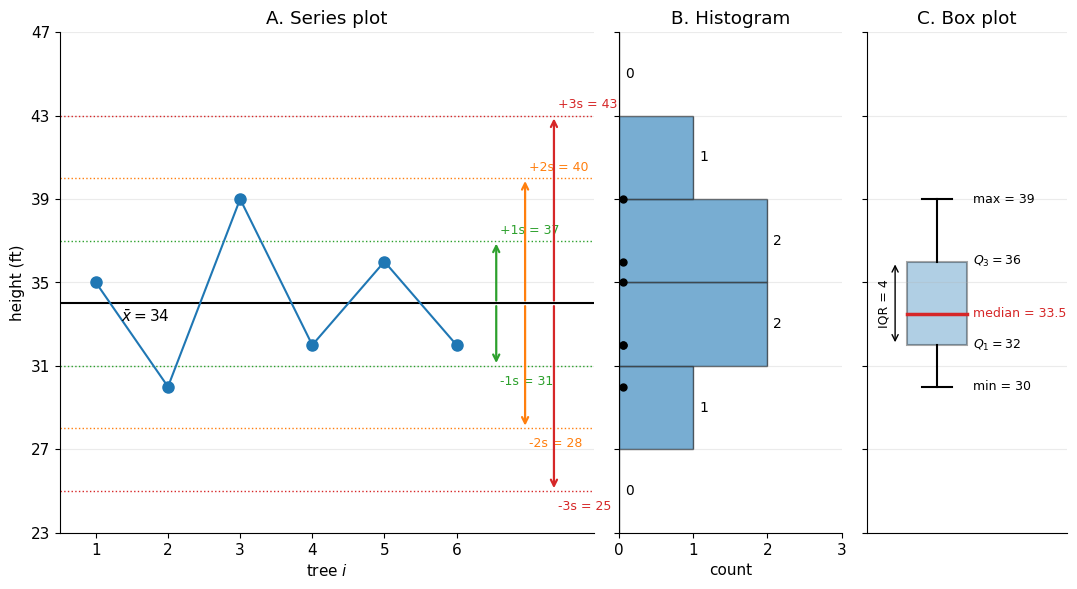
Draw three panels side by side sharing one vertical height axis from 23 to 47 ft: (A) series plot with \(\bar{x}\) and \(\pm 1s, \pm 2s, \pm 3s\) arrows, (B) sideways histogram with 4 ft bins, (C) box plot.
Panel A table. Fill in \(\bar{x} \pm ks\).
| \(\bar{x} - ks\) | \(\bar{x} + ks\) | |
|---|---|---|
| \(k = 1\) | ||
| \(k = 2\) | ||
| \(k = 3\) |
Answer. With \(\bar{x} = 34\) and \(s = 3\):
| \(\bar{x} - ks\) | \(\bar{x} + ks\) | |
|---|---|---|
| \(k = 1\) | \(34 - 3 = 31\) | \(34 + 3 = 37\) |
| \(k = 2\) | \(34 - 6 = 28\) | \(34 + 6 = 40\) |
| \(k = 3\) | \(34 - 9 = 25\) | \(34 + 9 = 43\) |
(a) How many points fall within \(\pm 1s\) of the mean?
Answer. Interval \([31, 37]\): \(x = 35, 32, 36, 32\) fall inside, so 4 points (\(i = 1, 4, 5, 6\)). Trees 2 (30 ft) and 3 (39 ft) fall outside. That is \(4/6 \approx 67\%\), close to the \(\approx 68\%\) expected for a normal distribution.
(b) How many points fall within \(\pm 2s\) of the mean?
Answer. Interval \([28, 40]\): all 6 points (\(100\%\); a normal distribution predicts \(\approx 95\%\)).
Panel B table. Count per bin (\([a, b)\) means \(a \le x < b\)).
| Bin (ft) | [23, 27) | [27, 31) | [31, 35) | [35, 39) | [39, 43) | [43, 47) |
|---|---|---|---|---|---|---|
| Count |
Answer. 30 goes in \([27,31)\); 32, 32 in \([31,35)\); 35 and 36 in \([35,39)\) (35 is on a boundary, so it goes up); 39 in \([39,43)\) (boundary, goes up).
| Bin (ft) | [23, 27) | [27, 31) | [31, 35) | [35, 39) | [39, 43) | [43, 47) |
|---|---|---|---|---|---|---|
| Count | 0 | 1 | 2 | 2 | 1 | 0 |
Total \(= 0 + 1 + 2 + 2 + 1 + 0 = 6 = N\).
Panel C. (c) Compute \(Q_1\), the median, \(Q_3\), and the IQR.
Answer. Sorted: \(\underbrace{30,\ 32,\ 32}_{\text{lower half}},\ \underbrace{35,\ 36,\ 39}_{\text{upper half}}\)
\[ \begin{aligned} Q_1 &= \text{median}(30, 32, 32) = 32 \text{ ft} \\ Q_2 &= \text{median} = \frac{32 + 35}{2} = 33.5 \text{ ft} \\ Q_3 &= \text{median}(35, 36, 39) = 36 \text{ ft} \\ \text{IQR} &= Q_3 - Q_1 = 36 - 32 = 4 \text{ ft} \end{aligned} \]
(d) What percent of the data lies inside the box?
Answer. The box spans \([32, 36]\) and contains \(32, 32, 35, 36\):
\[ \frac{4}{6} \approx 67\% \]
(By design the box holds roughly the middle 50%; with only \(N = 6\) and points sitting on the box edges, the actual fraction is 4 of 6.)
(e) What does the series plot show that the histogram and box plot do not?
Answer. The series plot keeps the identity and order of each observation (which tree \(i\) has which height). The histogram and box plot collapse the data into a distribution, so you can no longer tell which tree is which or see any trend or pattern across \(i\).
1.7 Normalized histogram and the normal PDF
Bin width \(\Delta = 4\) ft; \(c_k\) is the center of bin \(k\).
| Bin (ft) | \(c_k\) | Count | \(p_k = \text{count}/N\) | \(h_k = p_k/\Delta\) | \(f(c_k)\) (given) |
|---|---|---|---|---|---|
| [23, 27) | 25 | 0.004 | |||
| [27, 31) | 29 | 0.032 | |||
| [31, 35) | 33 | 0.088 | |||
| [35, 39) | 37 | 0.088 | |||
| [39, 43) | 41 | 0.032 | |||
| [43, 47) | 45 | 0.004 | |||
| Sum |
Answer. Completed table (\(N = 6\), \(\Delta = 4\)):
| Bin (ft) | \(c_k\) | Count | \(p_k = \text{count}/6\) | \(h_k = p_k/4\) (1/ft) | \(f(c_k)\) (given) |
|---|---|---|---|---|---|
| [23, 27) | 25 | 0 | \(0\) | \(0\) | 0.004 |
| [27, 31) | 29 | 1 | \(1/6 \approx 0.167\) | \(1/24 \approx 0.042\) | 0.032 |
| [31, 35) | 33 | 2 | \(1/3 \approx 0.333\) | \(1/12 \approx 0.083\) | 0.088 |
| [35, 39) | 37 | 2 | \(1/3 \approx 0.333\) | \(1/12 \approx 0.083\) | 0.088 |
| [39, 43) | 41 | 1 | \(1/6 \approx 0.167\) | \(1/24 \approx 0.042\) | 0.032 |
| [43, 47) | 45 | 0 | \(0\) | \(0\) | 0.004 |
| Sum | 6 | 1 | 1/4 = 0.25 | 0.248 |
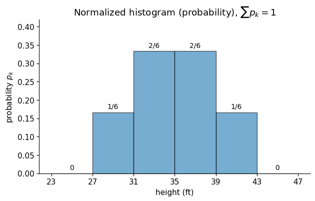
(a) Fill in \(p_k\) and draw these bars. Compute \(\sum p_k\).
Answer.
\[ \sum_{k} p_k = 0 + \frac{1}{6} + \frac{2}{6} + \frac{2}{6} + \frac{1}{6} + 0 = \frac{6}{6} = 1 \]
(b) Why must \(\sum p_k\) equal this value?
Answer. Every tree lands in exactly one bin, so the counts add up to \(N\) and the fractions add up to \(N/N = 1\). Equivalently, the probability that a tree falls in some bin is 100%.
(c) Fill in \(h_k\) and draw the density bars on a new plot. State the units of density.
Answer. \(h_k = p_k / \Delta\):
\[ \begin{aligned} h_{[27,31)} = h_{[39,43)} &= \frac{1/6}{4} = \frac{1}{24} \approx 0.042 \text{ ft}^{-1} \\ h_{[31,35)} = h_{[35,39)} &= \frac{1/3}{4} = \frac{1}{12} \approx 0.083 \text{ ft}^{-1} \\ h_{[23,27)} = h_{[43,47)} &= 0 \end{aligned} \]
Units of density: 1/ft (probability per foot).
The density bars and the PDF from part (d) are plotted together below.
(d) Plot the given \(f(c_k)\) at each bin center on the density plot and connect them with a smooth curve. Do the bars and curve roughly match? Would the match improve with 600 trees?
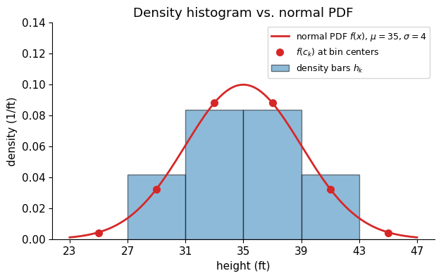
Answer. Yes, they roughly match: both are symmetric, tallest in the two middle bins (\(0.083\) vs. \(0.088\)), smaller in the next bins out (\(0.042\) vs. \(0.032\)), and near zero at the edges. With 600 trees the match would improve substantially, since the bin fractions converge to the true bin probabilities as \(N\) grows (law of large numbers); with \(N = 6\) each tree moves a bar by a large jump of \(1/24\).
(e) Riemann sum: compute \(\sum_{k=1}^{6} f(c_k)\,\Delta\), the approximate area under the PDF.
Answer.
\[ \begin{aligned} \sum_{k=1}^{6} f(c_k)\,\Delta &= 4\left(0.004 + 0.032 + 0.088 + 0.088 + 0.032 + 0.004\right) \\ &= 4\,(0.248) \\ &= 0.992 \approx 1 \end{aligned} \]
(Slightly under 1 because of the coarse bins and the small tails beyond 23 and 47 ft.)
(f) Compute \(\sum_k h_k\,\Delta\), the area of your density bars.
Answer.
\[ \begin{aligned} \sum_k h_k\,\Delta &= 4\left(0 + \tfrac{1}{24} + \tfrac{1}{12} + \tfrac{1}{12} + \tfrac{1}{24} + 0\right) \\ &= 4 \cdot \tfrac{6}{24} = 4 \cdot \tfrac{1}{4} \\ &= 1 \end{aligned} \]
(Exactly 1, since \(h_k \Delta = p_k\) and \(\sum p_k = 1\).)
(g) Explain intuitively why the area under a density curve equals 1.
Answer. Area under a density over an interval is the probability of landing in that interval (probability \(=\) density \(\times\) width). The whole curve covers every possible value, and the probability that a tree has some height is 100%, so the total area must be 1.
Part 2: Bivariate (two variables)
Setup. The forester also measures trunk diameter on the same six trees. Reuse all Part 1 results for \(X_1\).
| \(i\) | 1 | 2 | 3 | 4 | 5 | 6 |
|---|---|---|---|---|---|---|
| \(X_1\): Height (ft) | 35 | 30 | 39 | 32 | 36 | 32 |
| \(X_2\): Trunk diameter (in) | 11 | 7 | 13 | 8 | 10 | 11 |
2.1 Mean of \(X_2\)
Compute \(\bar{x}_2\).
Answer.
\[ \begin{aligned} \bar{x}_2 &= \frac{1}{6}\left(11 + 7 + 13 + 8 + 10 + 11\right) \\ &= \frac{60}{6} \\ &= 10 \text{ in} \end{aligned} \]
2.2 Deviations
\(d_{1,i} = x_{1,i} - \bar{x}_1\) and \(d_{2,i} = x_{2,i} - \bar{x}_2\). Fill in the table.
Answer. Using \(\bar{x}_1 = 34\) ft and \(\bar{x}_2 = 10\) in:
| \(i\) | \(x_{1,i}\) | \(x_{2,i}\) | \(d_{1,i}\) | \(d_{2,i}\) | \(d_{1,i}^2\) | \(d_{2,i}^2\) | \(d_{1,i}\,d_{2,i}\) |
|---|---|---|---|---|---|---|---|
| 1 | 35 | 11 | 1 | 1 | 1 | 1 | \((1)(1) = 1\) |
| 2 | 30 | 7 | \(-4\) | \(-3\) | 16 | 9 | \((-4)(-3) = 12\) |
| 3 | 39 | 13 | 5 | 3 | 25 | 9 | \((5)(3) = 15\) |
| 4 | 32 | 8 | \(-2\) | \(-2\) | 4 | 4 | \((-2)(-2) = 4\) |
| 5 | 36 | 10 | 2 | 0 | 4 | 0 | \((2)(0) = 0\) |
| 6 | 32 | 11 | \(-2\) | 1 | 4 | 1 | \((-2)(1) = -2\) |
| Sum | 204 | 60 | 0 | 0 | 54 | 24 | 30 |
2.3 Standard deviations
(a) Write \(s_1\) (from Part 1) and compute \(s_2\).
Answer.
\[ \begin{aligned} s_1 &= \sqrt{\frac{54}{6}} = \sqrt{9} = 3 \text{ ft} \quad \text{(from Part 1)} \\[4pt] s_2 &= \sqrt{\frac{1}{6}\left(1 + 9 + 9 + 4 + 0 + 1\right)} = \sqrt{\frac{24}{6}} = \sqrt{4} = 2 \text{ in} \end{aligned} \]
(b) State the units of \(s_1\) and \(s_2\).
Answer. \(s_1\): ft. \(s_2\): in.
2.4 Covariance
\(\text{cov}(X_1, X_2) = \frac{1}{N}\sum_{i=1}^{N} d_{1,i}\,d_{2,i}\)
(a) Compute the covariance.
Answer.
\[ \begin{aligned} \text{cov}(X_1, X_2) &= \frac{1}{6}\left(1 + 12 + 15 + 4 + 0 + (-2)\right) \\ &= \frac{30}{6} \\ &= 5 \text{ ft}\cdot\text{in} \end{aligned} \]
(b) State the units of the covariance.
Answer. ft\(\cdot\)in (feet times inches), the product of the two variables’ units.
(c) When is a product \(d_{1,i}\,d_{2,i}\) positive? Which tree contributes the largest product?
Answer. The product is positive when both deviations have the same sign: the tree is above the mean in both variables, or below the mean in both. Tree 3 contributes the largest product, \((5)(3) = 15\).
2.5 Pearson correlation coefficient
\(r = \dfrac{\text{cov}(X_1, X_2)}{s_1\, s_2}\)
(a) Compute \(r\).
Answer.
\[ \begin{aligned} r &= \frac{\text{cov}(X_1, X_2)}{s_1\,s_2} = \frac{5}{(3)(2)} \\ &= \frac{5}{6} \\ &\approx 0.83 \end{aligned} \]
(b) What are the units of \(r\)? Explain why, using the units of the numerator and denominator.
Answer. \(r\) is unitless:
\[ [r] = \frac{\text{ft}\cdot\text{in}}{\text{ft}\cdot\text{in}} = 1 \]
The covariance (numerator) has units ft\(\cdot\)in, and \(s_1 s_2\) (denominator) also has units ft\(\cdot\)in, so they cancel. This is why \(r\) does not change if we switch to meters or centimeters.
(c) Between what two values must \(r\) always lie?
Answer. \(-1 \le r \le 1\).
(d) Describe the relationship: strong or weak, positive or negative?
Answer. Strong positive (\(r \approx 0.83\)): taller trees tend to have thicker trunks.
2.6 Stacked series plot
Stack two plots vertically sharing one horizontal axis \(i = 1, \dots, 6\): height on top, trunk diameter below. In each, draw the mean as a horizontal line and an arrow from the mean to each point (its deviation).
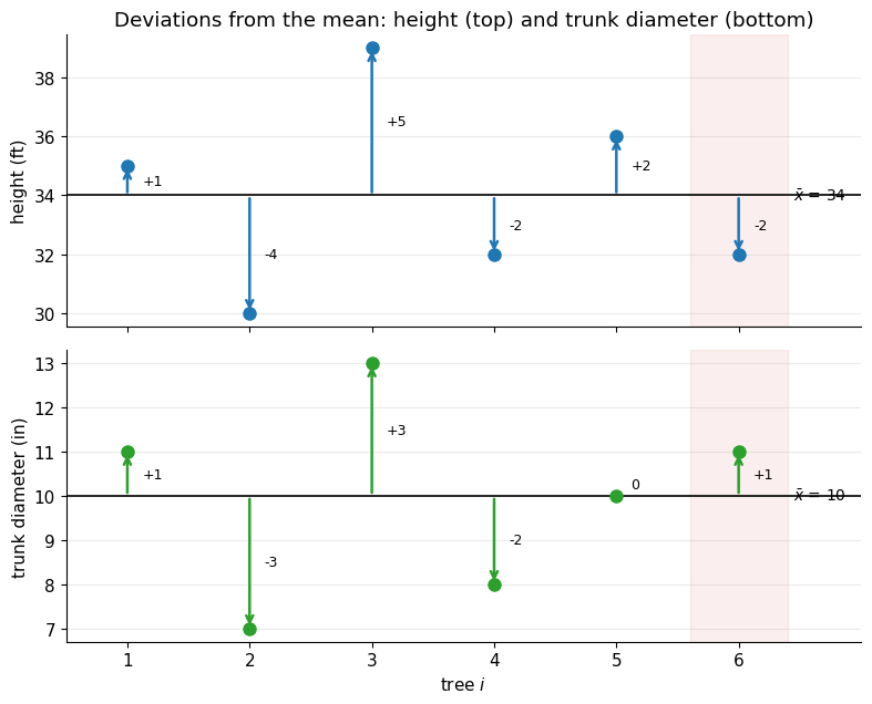
(a) For how many trees do the two arrows point the same direction (or one is zero)? Which tree breaks the pattern?
Answer. 5 trees (\(i = 1, 2, 3, 4\) same direction; \(i = 5\) has a zero diameter deviation). Tree 6 breaks the pattern: below-mean height (\(-2\)) but above-mean diameter (\(+1\)).
(b) How does this relate to the sign of the covariance?
Answer. When the arrows point the same way, \(d_{1,i}d_{2,i} > 0\). Since 4 trees give positive products (1, 12, 15, 4), one gives 0, and only tree 6 gives a small negative product (\(-2\)), the sum is positive (\(30\)), so the covariance is positive (\(5\) ft\(\cdot\)in). Tree 6 pulls it down slightly, which is one reason \(r < 1\).
2.7 Pair plot (2 × 2)
\(X_1\) bins: [27, 31), [31, 35), [35, 39), [39, 43). \(X_2\) bins: [6, 8), [8, 10), [10, 12), [12, 14). Write \(r\) on both scatter plots.
| Column \(X_1\) | Column \(X_2\) | |
|---|---|---|
| Row \(X_1\) | Histogram of \(X_1\) | Scatter: horizontal \(X_2\), vertical \(X_1\) |
| Row \(X_2\) | Scatter: horizontal \(X_1\), vertical \(X_2\) | Histogram of \(X_2\) |
Answer. Bin counts used for the diagonal histograms:
| \(X_1\) bin (ft) | [27, 31) | [31, 35) | [35, 39) | [39, 43) |
|---|---|---|---|---|
| Count | 1 | 2 | 2 | 1 |
| \(X_2\) bin (in) | [6, 8) | [8, 10) | [10, 12) | [12, 14) |
|---|---|---|---|---|
| Count | 1 | 1 | 3 | 1 |
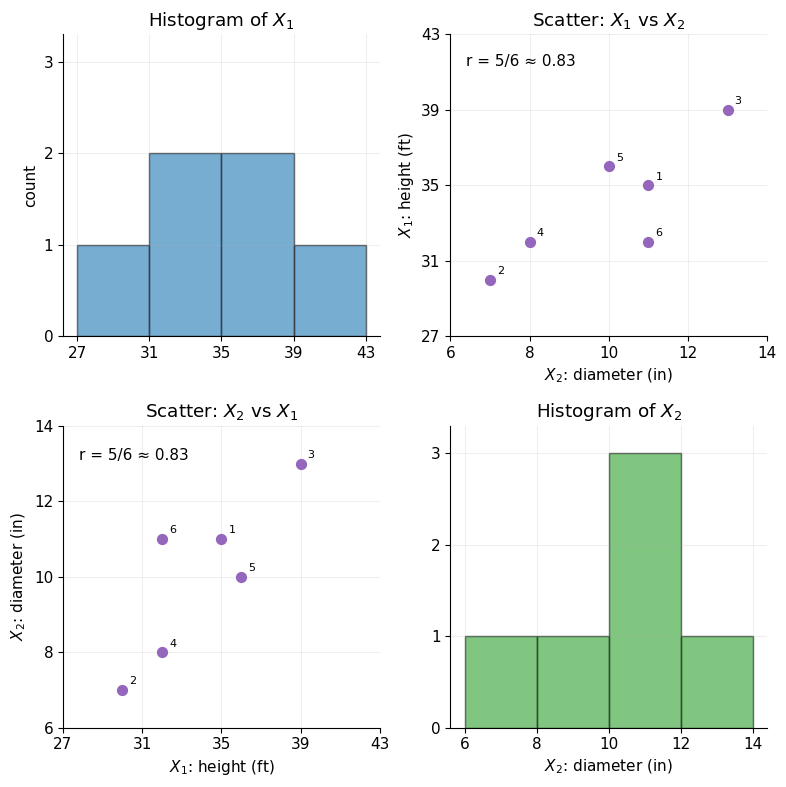
(a) Do the diagonal histograms show marginal or joint distributions?
Answer. Marginal distributions: each shows one variable alone, ignoring the other.
(b) How are the two scatter plots related to each other?
Answer. They contain the same six points with the axes swapped, so each is the mirror image (transpose) of the other, reflected across the diagonal line \(X_1 = X_2\). They carry identical information and the same \(r = 5/6\).
2.8 2D histogram (heat map)
Place each tree in its cell, write the count in every cell (including 0), then redraw the grid shading cells darker for higher counts.
| \(X_2\) bin \(X_1\) bin | [27, 31) | [31, 35) | [35, 39) | [39, 43) |
|---|---|---|---|---|
| [12, 14) | ||||
| [10, 12) | ||||
| [8, 10) | ||||
| [6, 8) |
Answer. Cell assignments \((x_1, x_2)\):
- Tree 1 \((35, 11)\): \(X_1 \in [35,39)\), \(X_2 \in [10,12)\)
- Tree 2 \((30, 7)\): \(X_1 \in [27,31)\), \(X_2 \in [6,8)\)
- Tree 3 \((39, 13)\): \(X_1 \in [39,43)\), \(X_2 \in [12,14)\)
- Tree 4 \((32, 8)\): \(X_1 \in [31,35)\), \(X_2 \in [8,10)\)
- Tree 5 \((36, 10)\): \(X_1 \in [35,39)\), \(X_2 \in [10,12)\)
- Tree 6 \((32, 11)\): \(X_1 \in [31,35)\), \(X_2 \in [10,12)\)
| \(X_2\) bin \(X_1\) bin | [27, 31) | [31, 35) | [35, 39) | [39, 43) |
|---|---|---|---|---|
| [12, 14) | 0 | 0 | 0 | 1 |
| [10, 12) | 0 | 1 | 2 | 0 |
| [8, 10) | 0 | 1 | 0 | 0 |
| [6, 8) | 1 | 0 | 0 | 0 |
| Column sum | 1 | 2 | 2 | 1 |
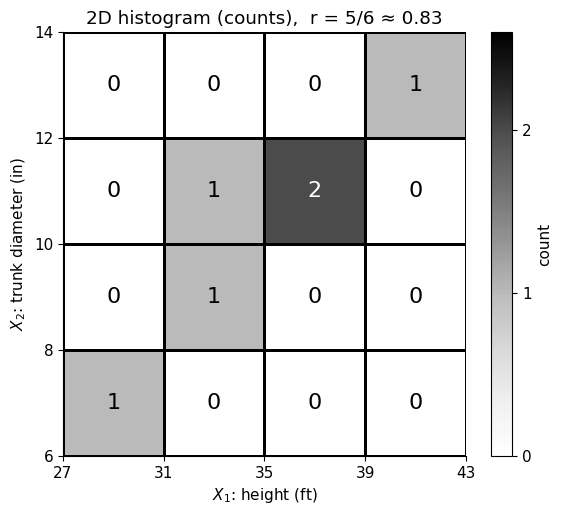
(a) Which cell has the highest count?
Answer. \(X_1 \in [35, 39)\) ft, \(X_2 \in [10, 12)\) in, with a count of 2 (trees 1 and 5).
(b) Describe the pattern of occupied cells and how it relates to \(r\).
Answer. The occupied cells run along the diagonal from lower left to upper right: short trees have thin trunks and tall trees have thick trunks, which is the positive relationship measured by \(r \approx 0.83\). The pattern is not a perfect diagonal (tree 6 sits one cell above it at \([31,35) \times [10,12)\)), consistent with \(r\) being strong but less than 1.
(c) What do you get by adding up each column of this grid?
Answer. Column sums \(= 1, 2, 2, 1\), which is exactly the marginal histogram of \(X_1\) (height) from the pair plot. Summing over the \(X_2\) bins removes that variable and leaves the distribution of \(X_1\) alone. (Likewise, row sums give the marginal histogram of \(X_2\): \(1, 1, 3, 1\).)