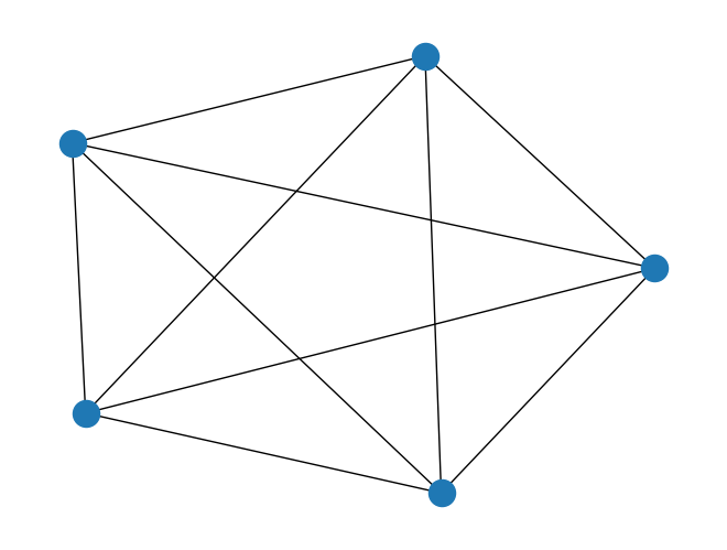
In the following self-contained example we show how to add various customization options to a plot
import networkx as nximport matplotlib.pyplot as plt#GENERATE GRAPHG = nx.complete_graph(5)print(type(G))# print(len(dir(G)))# [attr for attr in dir(G) if not callable(getattr(G, attr)) and not attr.startswith("__")]
<class 'networkx.classes.graph.Graph'>
#BASIC PLOTnx.draw(G)plt.show()
G = nx.complete_graph(10)
fig, ax = plt.subplots()print(type(ax))
<class 'matplotlib.axes._axes.Axes'>
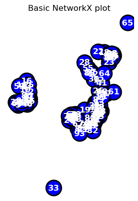
# G = nx.random_geometric_graph(100, 0.15)#CUSTOMIZE#specifiy x-y positions for plotting# pos=nx.circular_layout(G)pos=nx.spring_layout(G)# print degree of each nodefor node in G.nodes():print(f"Node {node} has degree {G.degree(node)}")#initialize plotfig, ax = plt.subplots()nx.draw(G,node_color='blue',edgecolors="black",edge_color="black", linewidths=2,font_color="white",font_weight="bold",node_size=500,width=2,with_labels=True,pos=pos,ax=ax)ax.set(title='Basic NetworkX plot')ax.set_aspect('equal', 'box')#fig.savefig("test.png")plt.show()
Node 0 has degree 7
Node 1 has degree 10
Node 2 has degree 8
Node 3 has degree 6
Node 4 has degree 9
Node 5 has degree 5
Node 6 has degree 9
Node 7 has degree 7
Node 8 has degree 5
Node 9 has degree 10
Node 10 has degree 6
Node 11 has degree 9
Node 12 has degree 5
Node 13 has degree 5
Node 14 has degree 3
Node 15 has degree 8
Node 16 has degree 2
Node 17 has degree 5
Node 18 has degree 3
Node 19 has degree 4
Node 20 has degree 5
Node 21 has degree 7
Node 22 has degree 1
Node 23 has degree 6
Node 24 has degree 4
Node 25 has degree 3
Node 26 has degree 9
Node 27 has degree 4
Node 28 has degree 1
Node 29 has degree 10
Node 30 has degree 5
Node 31 has degree 8
Node 32 has degree 9
Node 33 has degree 0
Node 34 has degree 5
Node 35 has degree 9
Node 36 has degree 9
Node 37 has degree 5
Node 38 has degree 7
Node 39 has degree 8
Node 40 has degree 7
Node 41 has degree 4
Node 42 has degree 5
Node 43 has degree 9
Node 44 has degree 12
Node 45 has degree 9
Node 46 has degree 5
Node 47 has degree 8
Node 48 has degree 7
Node 49 has degree 7
Node 50 has degree 7
Node 51 has degree 9
Node 52 has degree 11
Node 53 has degree 10
Node 54 has degree 6
Node 55 has degree 4
Node 56 has degree 7
Node 57 has degree 4
Node 58 has degree 9
Node 59 has degree 2
Node 60 has degree 8
Node 61 has degree 1
Node 62 has degree 6
Node 63 has degree 5
Node 64 has degree 3
Node 65 has degree 0
Node 66 has degree 7
Node 67 has degree 8
Node 68 has degree 7
Node 69 has degree 6
Node 70 has degree 8
Node 71 has degree 11
Node 72 has degree 7
Node 73 has degree 11
Node 74 has degree 11
Node 75 has degree 6
Node 76 has degree 6
Node 77 has degree 7
Node 78 has degree 12
Node 79 has degree 11
Node 80 has degree 7
Node 81 has degree 7
Node 82 has degree 2
Node 83 has degree 4
Node 84 has degree 8
Node 85 has degree 7
Node 86 has degree 6
Node 87 has degree 9
Node 88 has degree 10
Node 89 has degree 10
Node 90 has degree 12
Node 91 has degree 7
Node 92 has degree 7
Node 93 has degree 3
Node 94 has degree 7
Node 95 has degree 11
Node 96 has degree 8
Node 97 has degree 4
Node 98 has degree 4
Node 99 has degree 5
Customizing a plot: Example-2
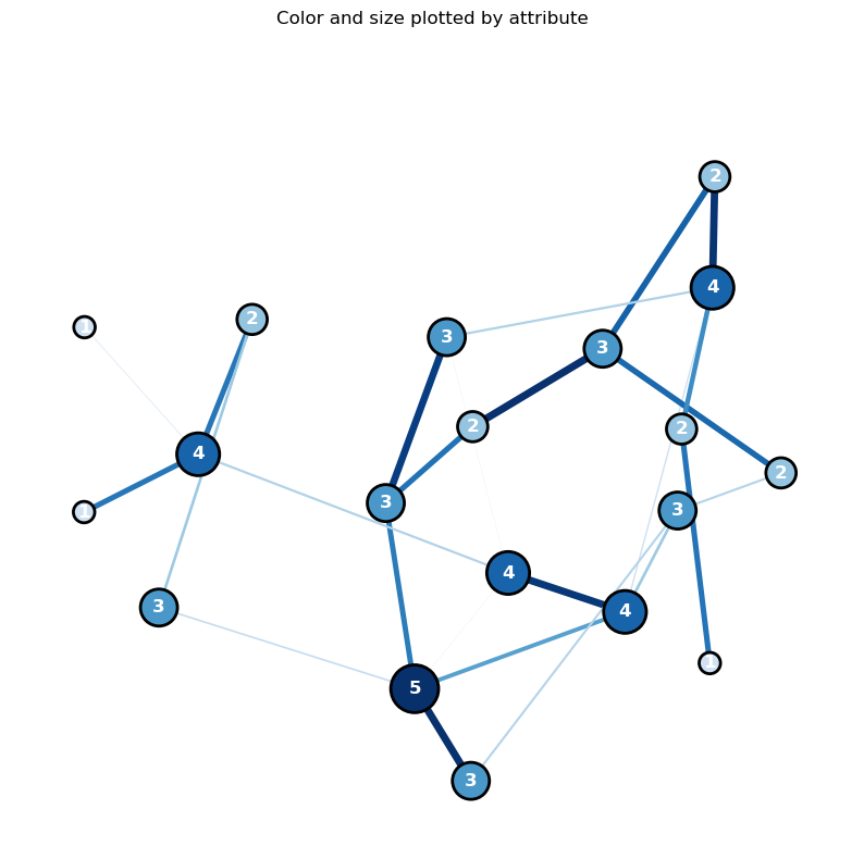
In the following self-contained example we show how to add various customization options to a NetworkX plot
import networkx as nximport matplotlib.pyplot as pltimport randomimport numpy as np#GENERATE GRAPHN=20G = nx.complete_graph(N)G = nx.gnp_random_graph(N, 0.1, seed=10374196)#ASSIGN RANDOM ATTRIBUTES TO NODES+EDGESfor u in G.nodes(): G.nodes[u]['x1']=0.2+1*random.uniform(0, 1) for u,v in G.edges(): G[u][v]['weight']=5*random.uniform(0, 1) print("here;",G.nodes[0]['x1'])#PRINT NODE+EDGESfor node in G.nodes(data=True): print(node)for line in nx.generate_edgelist(G, data=True): print(line)#SPECIFIY X-Y POSITIONS FOR PLOTTING# pos=nx.circular_layout(G)pos=nx.spring_layout(G,k=50*1./np.sqrt(N),iterations=500)# pos=nx.random_layout(G)#GENERATE PLOTfig, ax = plt.subplots()fig.set_size_inches(10, 10)#assign colors based on attributesweights_n = [G.nodes[u]['x1'] for u in G.nodes()]weights_e = [G[u][v]['weight'] for u,v in G.edges()]#SAMPLE CMAP FOR COLORS cmap=plt.cm.get_cmap('Blues')colors_e = [cmap(G[u][v]['weight']/5.0) for u,v in G.edges()]colors_n = [cmap(G.nodes[u]['x1']/1.2) for u in G.nodes()]#VARIOUS METHODS FOR VISUALIZING SIZE#LABELS (DICT)labels={}for n,d in nx.degree(G): labels[n]=d #str(n)+"-"+str(d) #WEIGHTS# node_size=1000*weights_n#DEGREE CENTRALITYcentrality=nx.degree(G)centrality=np.array([d for n,d in centrality]);#print(G_DEGREE)node_size=1000*centrality/max(centrality)colors_n = node_sizecolors_n = [cmap(u/max(centrality)) for u in centrality]#PLOTnx.draw(G, node_color=colors_n, edgecolors="black", edge_color=colors_e, linewidths=2, labels=labels, font_color="white", font_weight="bold", node_size=node_size, width=weights_e, with_labels=True, pos=pos, ax=ax)#TITLE ax.set(title='Color and size plotted by attribute')ax.set_aspect('equal', 'box')#PLOT# fig.savefig("test.png")plt.show()
/var/folders/lc/n91cn5z96ws6f52d25t2rpbh0000gn/T/ipykernel_83928/2489572329.py:36: MatplotlibDeprecationWarning: The get_cmap function was deprecated in Matplotlib 3.7 and will be removed in 3.11. Use ``matplotlib.colormaps[name]`` or ``matplotlib.colormaps.get_cmap()`` or ``pyplot.get_cmap()`` instead.
  cmap=plt.cm.get_cmap('Blues')
Node degree histogram
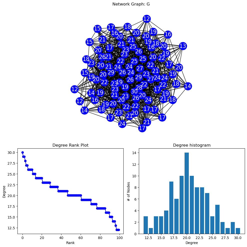
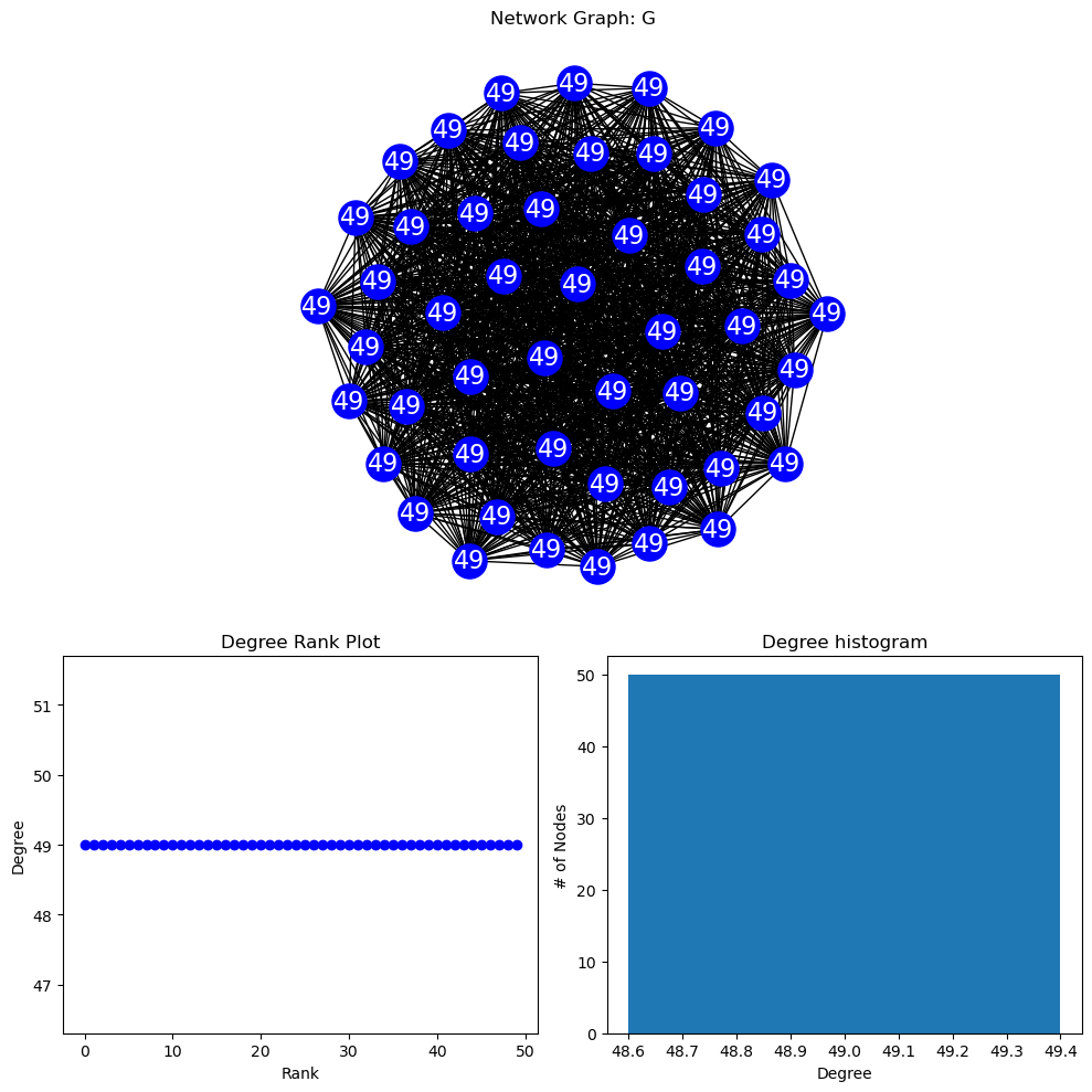
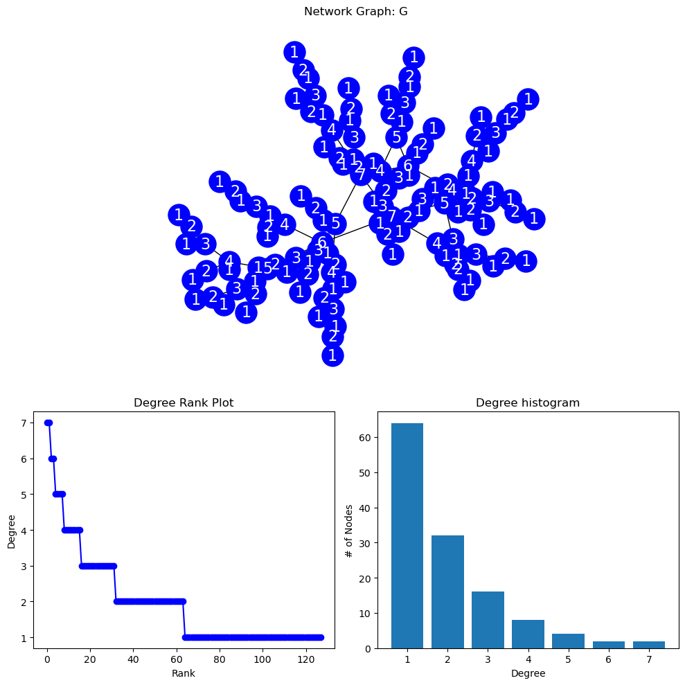
A node degree histogram is a graphical representation of the frequency distribution of the degrees of nodes in a network.
The x-axis shows the node degrees, and the y-axis displays the number of nodes with that degree.
It helps visualize the connectivity pattern of a network, such as the presence of hubs or the degree distribution.
# MODIFIED FROM # https://networkx.org/documentation/stable/auto_examples/drawing/plot_degree.htmlimport networkx as nximport numpy as npimport matplotlib.pyplot as plt#-------------------# PLOTTING FUNCTION#-------------------def degree_histogram_plot(G):#COMPUTE DEGREE: --> "LIST" WITH NODE DEGREES G_DEGREE=G.degree();#print(G_DEGREE,G_DEGREE[5],type(G_DEGREE)) #LABELS (DICT) labels={}for n,d in G_DEGREE: labels[n]=d #str(n)+"-"+str(d) #SORT DEGREE AND STORE IN LIST degree_sequence =sorted((d for n, d in G_DEGREE), reverse=True) dmax =max(degree_sequence) #MAX DEGREE#INITIALIZE MPL FIGURE+AX fig = plt.figure("Degree of a random graph", figsize=(10, 10))# Create a gridspec for adding subplots of different sizes axgrid = fig.add_gridspec(5, 4)#PLOT NETWORK IN UPPER GRID SPACES ax0 = fig.add_subplot(axgrid[0:3, :]) pos = nx.spring_layout(G) nx.draw(G, with_labels=True, labels=labels, node_color='blue', node_size=500, font_color='white', font_size=16, pos=pos,ax=ax0 ) ax0.set_title("Network Graph: G")#PLOT RANK (IMPORTANCE BASED ON DEGREE) VS DEGREE) ax1 = fig.add_subplot(axgrid[3:, :2]) ax1.plot(degree_sequence, "b-", marker="o") ax1.set_title("Degree Rank Plot") ax1.set_ylabel("Degree") ax1.set_xlabel("Rank")#PLOT RANK HISTOGRAM ax2 = fig.add_subplot(axgrid[3:, 2:]) ax2.bar(*np.unique(degree_sequence, return_counts=True)) ax2.set_title("Degree histogram") ax2.set_xlabel("Degree") ax2.set_ylabel("# of Nodes") ax0.set_aspect('equal', 'box') fig.tight_layout() plt.show()print("NETWORK DENSITY:", nx.density(G), "\n","NETWORK DIAMETER:", nx.diameter(G), "\n", )#-------------------#GENERATE GRAPHS+PLOT#-------------------print("RANDOM GRAPH")#gnp_random_graph(n, p=, seed=None, directed=False)#p=connection probablityG = nx.gnp_random_graph(100, 0.2, seed=10374196)degree_histogram_plot(G)print("COMPLETE GRAPH")G = nx.complete_graph(50)degree_histogram_plot(G)print("BINOMIAL TREE")G = nx.binomial_tree(7)degree_histogram_plot(G)
NETWORK DENSITY: 1.0
 NETWORK DIAMETER: 1

BINOMIAL TREE
NETWORK DENSITY: 0.015625
 NETWORK DIAMETER: 13
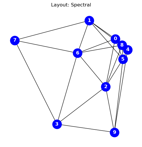
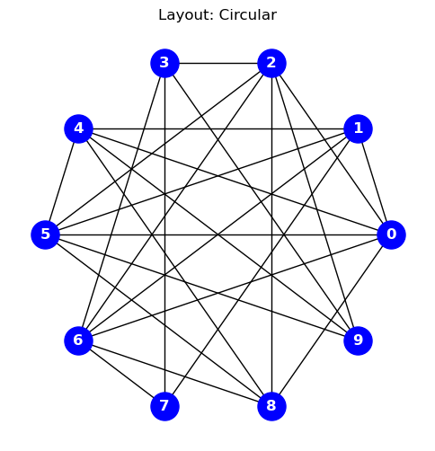
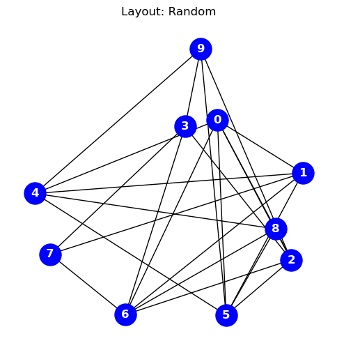
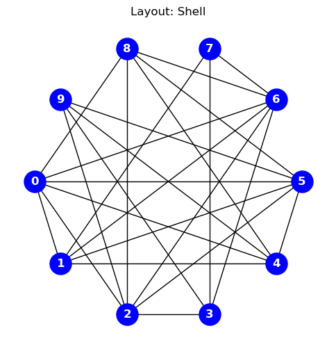
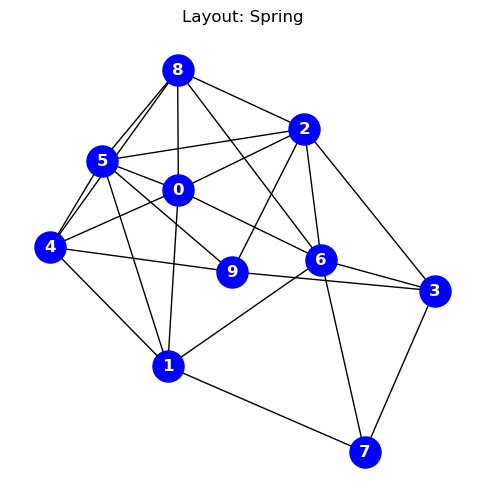
Graph Layouts
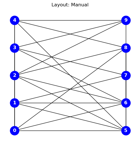
A graph visualization layout arranges nodes and edges in a visually intuitive manner.
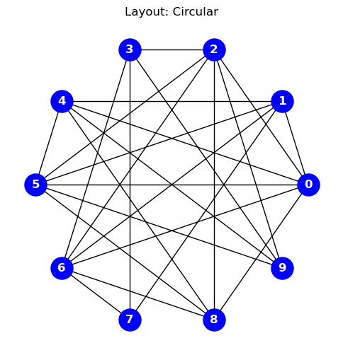
Examples include hierarchical trees with parent-child relationships, force-directed layouts where nodes repel each other, and circular layouts that arrange nodes in a circle.
In the following example the code explores various Network-X positional layouts
import networkx as nximport matplotlib.pyplot as plt#GENERATE A COMPLETE GRAPH USING A GRAPH GENERATOR #https://networkx.org/documentation/stable/reference/generators.html# G = nx.complete_graph(10)G = nx.gnp_random_graph(10,p=0.7)for i inrange(1,7+1):#print(i)#CAN MANUALLY SPECIFY GRAPH LOCATIONS WITH A DICTIONARY OF (X,Y) ARRAYS if(i==1): title="Layout: Manual"; pos={}; j=0; i1=0for k inrange(0,len(list(G.edges))):if(k%5==0): j=j+1if(k%5==0): i1=0 i1=i1+1 pos[k]=[j,i1]# OR YOU CAN USE ONE OF NETWORK-X'S BUILT-IN POSITION LAYOUT ALGORITHMSif(i==2): title="Layout: Spectral"; pos = nx.spectral_layout(G)if(i==3): title="Layout: Circular"; pos = nx.circular_layout(G)# if(i==4): title="Layout: Kamada-Kawai"; pos = nx.kamada_kawai_layout(G)if(i==5): title="Layout: Random"; pos = nx.random_layout(G)if(i==6): title="Layout: Shell"; pos = nx.shell_layout(G)if(i==7): title="Layout: Spring"; pos = nx.spring_layout(G,iterations=200) fig, ax = plt.subplots() fig.set_size_inches(6, 6) nx.draw( G, node_color="blue", node_size=500, font_color="white", font_weight="bold", with_labels=True, pos=pos, ) ax.set(title=title)# if(i>1): ax.set_aspect('equal', 'box') plt.title(title) plt.show()