Code
<class 'networkx.classes.graph.Graph'>In the following self-contained example we show how to add various customization options to a plot
<class 'networkx.classes.graph.Graph'>#
G = nx.random_geometric_graph(100, 0.15)
#CUSTOMIZE
#specifiy x-y positions for plotting
# pos=nx.circular_layout(G)
pos=nx.spring_layout(G)
# print degree of each node
for node in G.nodes():
print(f"Node {node} has degree {G.degree(node)}")
#initialize plot
fig, ax = plt.subplots()
nx.draw(
G,
node_color='blue',
edgecolors="black",
edge_color="black",
linewidths=2,
font_color="white",
font_weight="bold",
node_size=500,
width=2,
with_labels=True,
pos=pos,
ax=ax
)
ax.set(title='Basic NetworkX plot')
ax.set_aspect('equal', 'box')
#fig.savefig("test.png")
plt.show()Node 0 has degree 7
Node 1 has degree 10
Node 2 has degree 8
Node 3 has degree 6
Node 4 has degree 9
Node 5 has degree 5
Node 6 has degree 9
Node 7 has degree 7
Node 8 has degree 5
Node 9 has degree 10
Node 10 has degree 6
Node 11 has degree 9
Node 12 has degree 5
Node 13 has degree 5
Node 14 has degree 3
Node 15 has degree 8
Node 16 has degree 2
Node 17 has degree 5
Node 18 has degree 3
Node 19 has degree 4
Node 20 has degree 5
Node 21 has degree 7
Node 22 has degree 1
Node 23 has degree 6
Node 24 has degree 4
Node 25 has degree 3
Node 26 has degree 9
Node 27 has degree 4
Node 28 has degree 1
Node 29 has degree 10
Node 30 has degree 5
Node 31 has degree 8
Node 32 has degree 9
Node 33 has degree 0
Node 34 has degree 5
Node 35 has degree 9
Node 36 has degree 9
Node 37 has degree 5
Node 38 has degree 7
Node 39 has degree 8
Node 40 has degree 7
Node 41 has degree 4
Node 42 has degree 5
Node 43 has degree 9
Node 44 has degree 12
Node 45 has degree 9
Node 46 has degree 5
Node 47 has degree 8
Node 48 has degree 7
Node 49 has degree 7
Node 50 has degree 7
Node 51 has degree 9
Node 52 has degree 11
Node 53 has degree 10
Node 54 has degree 6
Node 55 has degree 4
Node 56 has degree 7
Node 57 has degree 4
Node 58 has degree 9
Node 59 has degree 2
Node 60 has degree 8
Node 61 has degree 1
Node 62 has degree 6
Node 63 has degree 5
Node 64 has degree 3
Node 65 has degree 0
Node 66 has degree 7
Node 67 has degree 8
Node 68 has degree 7
Node 69 has degree 6
Node 70 has degree 8
Node 71 has degree 11
Node 72 has degree 7
Node 73 has degree 11
Node 74 has degree 11
Node 75 has degree 6
Node 76 has degree 6
Node 77 has degree 7
Node 78 has degree 12
Node 79 has degree 11
Node 80 has degree 7
Node 81 has degree 7
Node 82 has degree 2
Node 83 has degree 4
Node 84 has degree 8
Node 85 has degree 7
Node 86 has degree 6
Node 87 has degree 9
Node 88 has degree 10
Node 89 has degree 10
Node 90 has degree 12
Node 91 has degree 7
Node 92 has degree 7
Node 93 has degree 3
Node 94 has degree 7
Node 95 has degree 11
Node 96 has degree 8
Node 97 has degree 4
Node 98 has degree 4
Node 99 has degree 5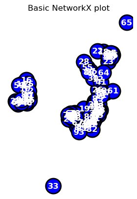
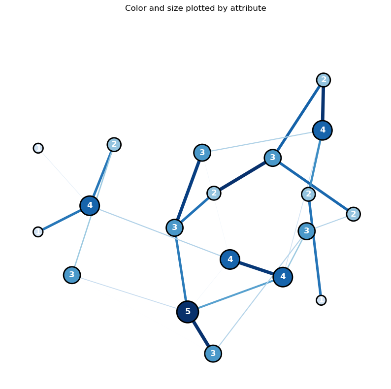
In the following self-contained example we show how to add various customization options to a NetworkX plot
import networkx as nx
import matplotlib.pyplot as plt
import random
import numpy as np

#GENERATE GRAPH
N=20

G = nx.complete_graph(N)
G = nx.gnp_random_graph(N, 0.1, seed=10374196)

#ASSIGN RANDOM ATTRIBUTES TO NODES+EDGES
for u in G.nodes(): G.nodes[u]['x1']=0.2+1*random.uniform(0, 1)
for u,v in G.edges(): G[u][v]['weight']=5*random.uniform(0, 1)

print("here;",G.nodes[0]['x1'])

#PRINT NODE+EDGES
for node in G.nodes(data=True): print(node)
for line in nx.generate_edgelist(G, data=True): print(line)

#SPECIFIY X-Y POSITIONS FOR PLOTTING
# pos=nx.circular_layout(G)
pos=nx.spring_layout(G,k=50*1./np.sqrt(N),iterations=500)
# pos=nx.random_layout(G)

#GENERATE PLOT
fig, ax = plt.subplots()
fig.set_size_inches(10, 10)

#assign colors based on attributes
weights_n   = [G.nodes[u]['x1'] for u in G.nodes()]
weights_e   = [G[u][v]['weight'] for u,v in G.edges()]

#SAMPLE CMAP FOR COLORS
cmap=plt.cm.get_cmap('Blues')
colors_e    = [cmap(G[u][v]['weight']/5.0) for u,v in G.edges()]
colors_n    = [cmap(G.nodes[u]['x1']/1.2) for u in G.nodes()]

#VARIOUS METHODS FOR VISUALIZING SIZE

#LABELS (DICT)
labels={}
for n,d in nx.degree(G): labels[n]=d #str(n)+"-"+str(d)

#WEIGHTS
# node_size=1000*weights_n

#DEGREE CENTRALITY
centrality=nx.degree(G)
centrality=np.array([d for n,d in centrality]); #print(G_DEGREE)
node_size=1000*centrality/max(centrality)
colors_n = node_size
colors_n = [cmap(u/max(centrality)) for u in centrality]

#PLOT
nx.draw(
G,
    node_color=colors_n,
    edgecolors="black",
    edge_color=colors_e,
    linewidths=2,
    labels=labels,
    font_color="white",
    font_weight="bold",
    node_size=node_size,
    width=weights_e,
    with_labels=True,
    pos=pos,
    ax=ax
)

#TITLE
ax.set(title='Color and size plotted by attribute')
ax.set_aspect('equal', 'box')

#PLOT
# fig.savefig("test.png")
plt.show()
here; 1.10843474533638
(0, {'x1': 1.10843474533638})
(1, {'x1': 0.4754941738266116})
(2, {'x1': 0.2595166365699992})
(3, {'x1': 0.774394122932119})
(4, {'x1': 0.655993848278551})
(5, {'x1': 0.8820701288233859})
(6, {'x1': 1.1326352281483743})
(7, {'x1': 1.048487098602679})
(8, {'x1': 0.28600734440670356})
(9, {'x1': 0.44088127010842676})
(10, {'x1': 0.6085487439097328})
(11, {'x1': 0.6484518385615652})
(12, {'x1': 1.0536148116095452})
(13, {'x1': 1.0688284842214122})
(14, {'x1': 1.1947753836726505})
(15, {'x1': 0.8003139376414383})
(16, {'x1': 0.6570813265223456})
(17, {'x1': 0.6018638893708343})
(18, {'x1': 0.4869168216168815})
(19, {'x1': 1.0776268479736169})
0 14 {'weight': 3.6315963677066905}
1 14 {'weight': 0.6169420542174209}
2 9 {'weight': 4.969913102796307}
2 11 {'weight': 3.712342132166846}
3 9 {'weight': 4.0342131124422504}
3 12 {'weight': 4.905915186238567}
4 11 {'weight': 4.7193967719742815}
4 12 {'weight': 1.59581420218815}
4 15 {'weight': 0.3140312659851291}
5 12 {'weight': 1.0085532001354713}
5 13 {'weight': 2.7893837047511907}
5 15 {'weight': 4.831202571973552}
5 17 {'weight': 1.8934566665404073}
6 19 {'weight': 3.67404154655943}
7 14 {'weight': 3.625428541128064}
7 18 {'weight': 1.8935531482497159}
8 9 {'weight': 3.9063111257647782}
8 17 {'weight': 1.5119606365198468}
10 13 {'weight': 4.960878646603789}
10 17 {'weight': 1.5063743482310739}
10 18 {'weight': 0.01641612853155172}
11 13 {'weight': 3.550941180208129}
12 19 {'weight': 3.205217480603006}
13 15 {'weight': 0.34503938879875073}
13 18 {'weight': 1.211262320380884}
14 15 {'weight': 1.5686710357555667}# MODIFIED FROM
# https://networkx.org/documentation/stable/auto_examples/drawing/plot_degree.html
import networkx as nx
import numpy as np
import matplotlib.pyplot as plt
#-------------------
# PLOTTING FUNCTION
#-------------------
def degree_histogram_plot(G):
#COMPUTE DEGREE: --> "LIST" WITH NODE DEGREES
G_DEGREE=G.degree(); #print(G_DEGREE,G_DEGREE[5],type(G_DEGREE))
#LABELS (DICT)
labels={}
for n,d in G_DEGREE: labels[n]=d #str(n)+"-"+str(d)
#SORT DEGREE AND STORE IN LIST
degree_sequence = sorted((d for n, d in G_DEGREE), reverse=True)
dmax = max(degree_sequence) #MAX DEGREE
#INITIALIZE MPL FIGURE+AX
fig = plt.figure("Degree of a random graph", figsize=(10, 10))
# Create a gridspec for adding subplots of different sizes
axgrid = fig.add_gridspec(5, 4)
#PLOT NETWORK IN UPPER GRID SPACES
ax0 = fig.add_subplot(axgrid[0:3, :])
pos = nx.spring_layout(G)
nx.draw(G,
with_labels=True,
labels=labels,
node_color='blue',
node_size=500,
font_color='white',
font_size=16,
pos=pos,ax=ax0
)
ax0.set_title("Network Graph: G")
#PLOT RANK (IMPORTANCE BASED ON DEGREE) VS DEGREE)
ax1 = fig.add_subplot(axgrid[3:, :2])
ax1.plot(degree_sequence, "b-", marker="o")
ax1.set_title("Degree Rank Plot")
ax1.set_ylabel("Degree")
ax1.set_xlabel("Rank")
#PLOT RANK HISTOGRAM
ax2 = fig.add_subplot(axgrid[3:, 2:])
ax2.bar(*np.unique(degree_sequence, return_counts=True))
ax2.set_title("Degree histogram")
ax2.set_xlabel("Degree")
ax2.set_ylabel("# of Nodes")
ax0.set_aspect('equal', 'box')
fig.tight_layout()
plt.show()
print(
"NETWORK DENSITY:", nx.density(G), "\n",
"NETWORK DIAMETER:", nx.diameter(G), "\n",
)
#-------------------
#GENERATE GRAPHS+PLOT
#-------------------
print("RANDOM GRAPH")
#gnp_random_graph(n, p=, seed=None, directed=False)
#p=connection probablity
G = nx.gnp_random_graph(100, 0.2, seed=10374196)
degree_histogram_plot(G)
print("COMPLETE GRAPH")
G = nx.complete_graph(50)
degree_histogram_plot(G)
print("BINOMIAL TREE")
G = nx.binomial_tree(7)
degree_histogram_plot(G)RANDOM GRAPH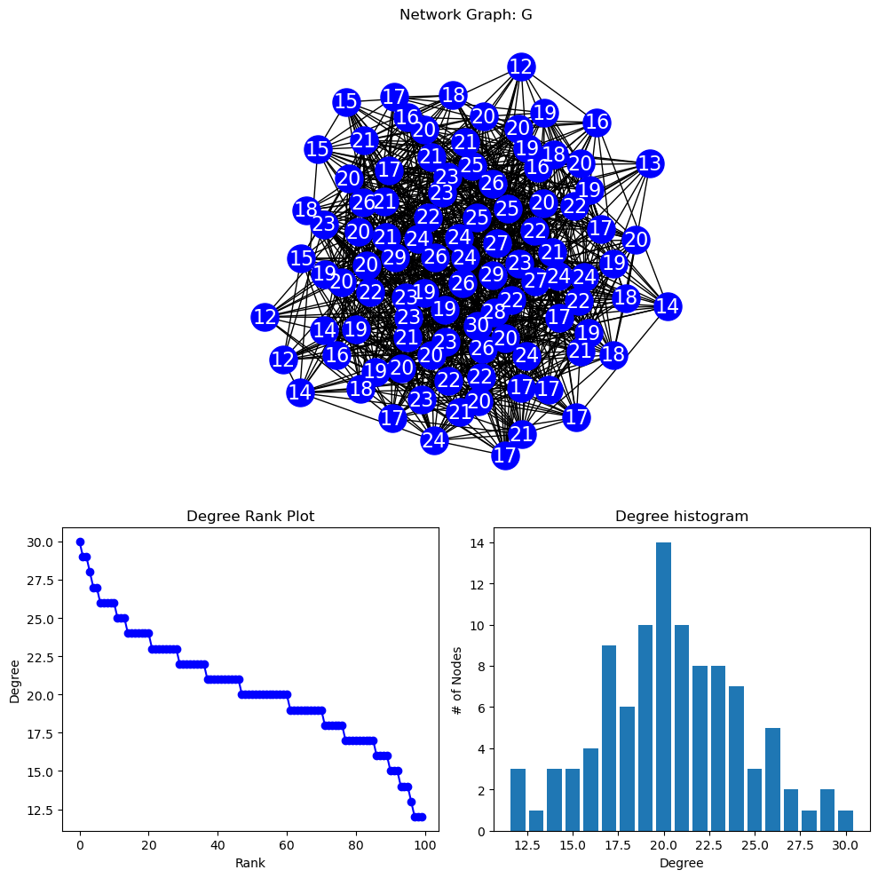
NETWORK DENSITY: 0.20646464646464646
 NETWORK DIAMETER: 3

COMPLETE GRAPH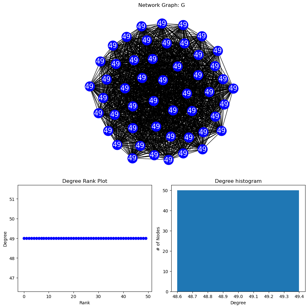
NETWORK DENSITY: 1.0
 NETWORK DIAMETER: 1

BINOMIAL TREE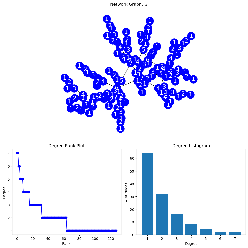
NETWORK DENSITY: 0.015625
 NETWORK DIAMETER: 13
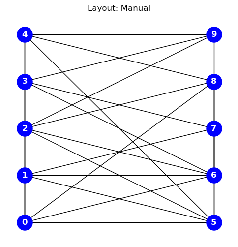
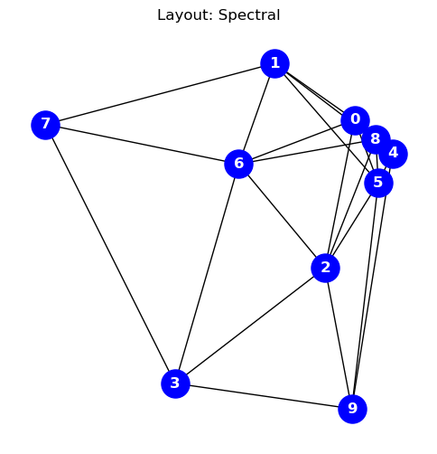
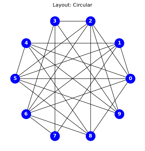
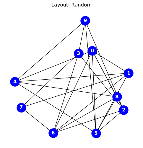
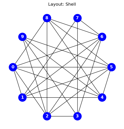
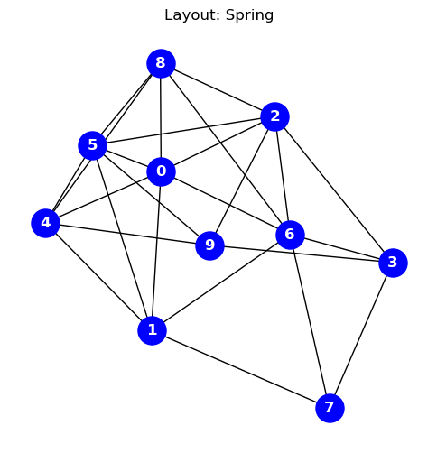
import networkx as nx
import matplotlib.pyplot as plt

#GENERATE A COMPLETE GRAPH USING A GRAPH GENERATOR
#https://networkx.org/documentation/stable/reference/generators.html
# G = nx.complete_graph(10)
G = nx.gnp_random_graph(10,p=0.7)
for i in range(1,7+1):
    #print(i)
    #CAN MANUALLY SPECIFY GRAPH LOCATIONS WITH A DICTIONARY OF (X,Y) ARRAYS
    if(i==1):
        title="Layout: Manual"; pos={}; j=0; i1=0
        for k in range(0,len(list(G.edges))):
            if(k%5==0): j=j+1
            if(k%5==0): i1=0
            i1=i1+1
            pos[k]=[j,i1]

    # OR YOU CAN USE ONE OF NETWORK-X'S BUILT-IN POSITION LAYOUT ALGORITHMS
    if(i==2): title="Layout: Spectral";     pos = nx.spectral_layout(G)
    if(i==3): title="Layout: Circular";     pos = nx.circular_layout(G)
    # if(i==4): title="Layout: Kamada-Kawai"; pos = nx.kamada_kawai_layout(G)
    if(i==5): title="Layout: Random";       pos = nx.random_layout(G)
    if(i==6): title="Layout: Shell";        pos = nx.shell_layout(G)
    if(i==7): title="Layout: Spring";       pos = nx.spring_layout(G,iterations=200)


    fig, ax = plt.subplots()
    fig.set_size_inches(6, 6)

    nx.draw(
        G,
        node_color="blue",
        node_size=500,
        font_color="white",
        font_weight="bold",
        with_labels=True,
        pos=pos,
    )
    ax.set(title=title)
    # if(i>1): ax.set_aspect('equal', 'box')
    plt.title(title)
    plt.show()