Code
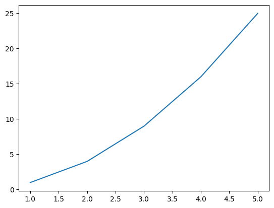
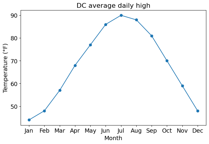
Matplotlib version: 3.10.8Three lines of code: give Matplotlib some x values, some y values, and ask it to draw.
What just happened?
plt.plot(x, y) connected the points (1,1), (2,4), ..., (5,25) with straight linesplt.show() rendered the figure
plt.show() is optional (but it hides extra text output, so it is a good habit).py script, plt.show() is required or nothing appearsx and y just need the same lengthEvery Matplotlib plot is built from two main objects:
ax.plot(), ax.set_xlabel(), ax.legend()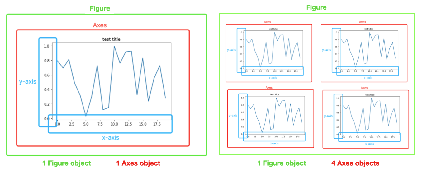
Watch the spelling:
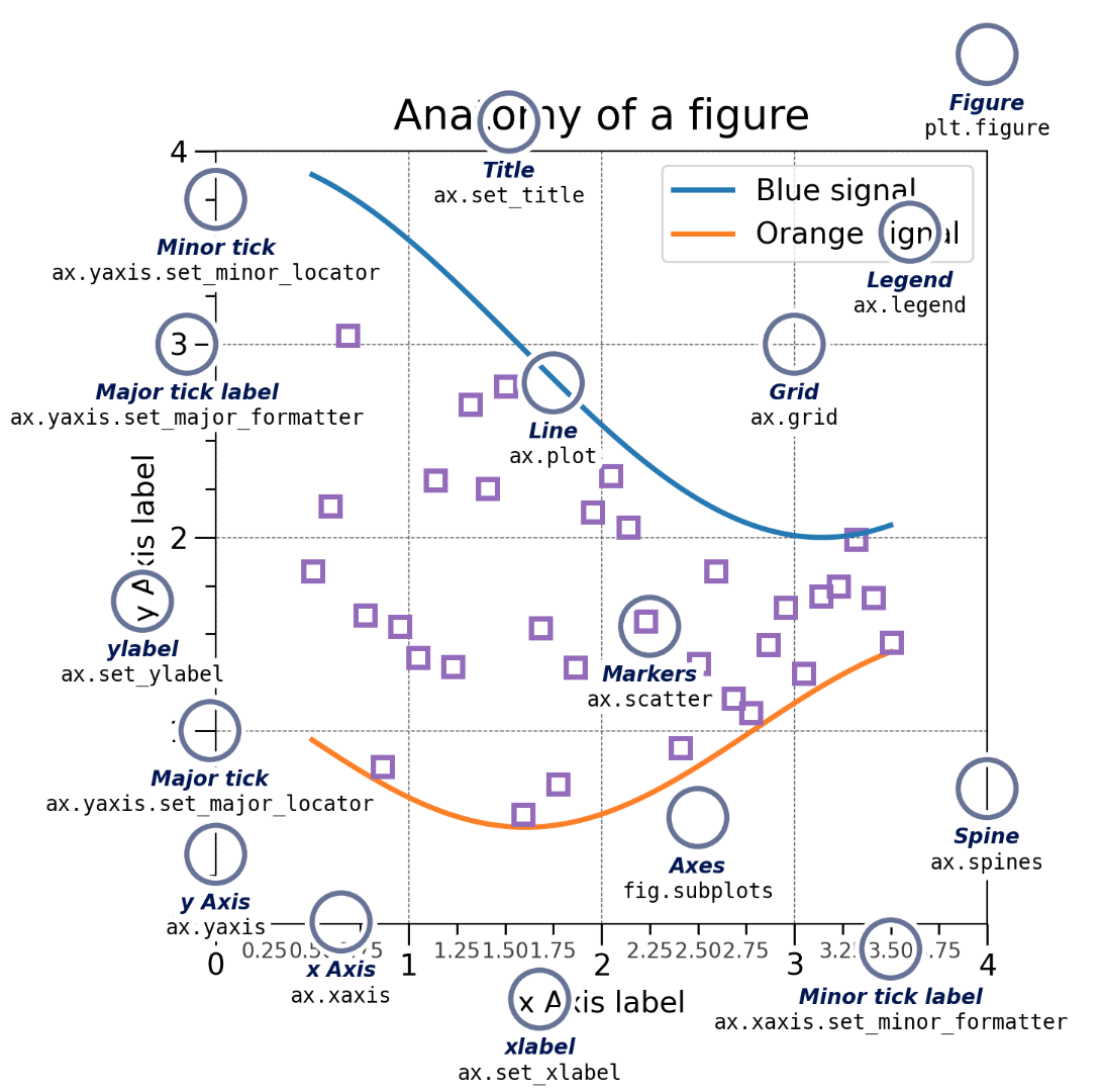
The labeled figure below names every component and the command that controls it. Keep it as a reference.
You will see both styles online, so you need to recognize both.
| Implicit (pyplot) style | Explicit (object-oriented) style | |
|---|---|---|
| How it works | plt silently tracks the “current” figure and Axes |
You create fig and ax and call methods on them |
| Looks like | plt.plot(), plt.xlabel() |
ax.plot(), ax.set_xlabel() |
| Good for | Very quick, throwaway plots | Everything else, especially multiple plots |
In this course we use the explicit style. It scales cleanly from one plot to many, and it is always clear which plot you are modifying.
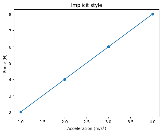
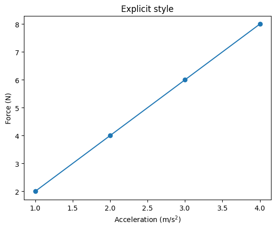
Same plot, slightly different names. Most Axes methods just add set_:
| pyplot | Axes method |
|---|---|
plt.title() |
ax.set_title() |
plt.xlabel() / plt.ylabel() |
ax.set_xlabel() / ax.set_ylabel() |
plt.xlim() / plt.ylim() |
ax.set_xlim() / ax.set_ylim() |
plt.xticks() |
ax.set_xticks() |
plt.plot(), plt.scatter(), plt.legend(), plt.grid() |
ax.plot(), ax.scatter(), ax.legend(), ax.grid() (same name) |
Tip: $...$ inside a label renders math (LaTeX), e.g. "m/s$^2$" becomes m/s².
Nearly every plot you ever make follows the same five steps. Memorize this template and reuse it.
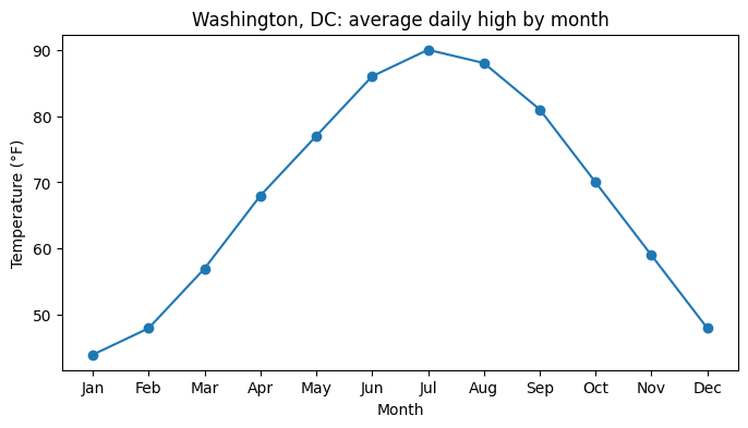
fig, ax = plt.subplots(figsize=(width, height)) (size in inches)ax.plot(...), ax.scatter(...), ax.bar(...), …fig.savefig(...), then plt.show()# 1. DATA: approximate average daily high temperature in Washington, DC
months = ["Jan", "Feb", "Mar", "Apr", "May", "Jun",
"Jul", "Aug", "Sep", "Oct", "Nov", "Dec"]
dc_high = [44, 48, 57, 68, 77, 86, 90, 88, 81, 70, 59, 48]
# 2. CREATE
fig, ax = plt.subplots(figsize=(8, 4))
# 3. PLOT
ax.plot(months, dc_high, marker="o")
# 4. LABEL
ax.set_title("Washington, DC: average daily high by month")
ax.set_xlabel("Month")
ax.set_ylabel("Temperature (°F)")
# 5. SAVE / SHOW
# fig.savefig("dc_temps.png", dpi=300, bbox_inches="tight") # (covered in Section 11)
plt.show()Notice that x can be text (the month names). Matplotlib treats them as ordered categories.
plt.subplots(nrows, ncols) creates a grid of Axes.
ax is a single Axes objectaxs[0], axs[1], …axs[row, col], e.g. axs[0, 1] is top row, second columnx = np.linspace(0, 2 * np.pi, 200)
fig, axs = plt.subplots(1, 2, figsize=(10, 3.5)) # 1 row, 2 columns
print(type(axs), axs.shape)
axs[0].plot(x, np.sin(x))
axs[0].set_title("sin(x)")
axs[1].plot(x, np.cos(x), color="tab:orange")
axs[1].set_title("cos(x)")
fig.suptitle("Two Axes in one Figure") # title for the whole Figure
plt.show()<class 'numpy.ndarray'> (2,)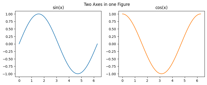
Three settings that make subplots look right:
layout="constrained": automatically spaces plots so labels never overlap (use it every time)sharex=True / sharey=True: subplots use the same axis range, which makes them directly comparablefor ax in axs.flat: loops over every Axes in a grid, so you can apply the same settings to all of themfuncs = [np.sin, np.cos, np.tanh, np.arctan]
names = ["sin(x)", "cos(x)", "tanh(x)", "arctan(x)"]
x = np.linspace(-3, 3, 400)
fig, axs = plt.subplots(2, 2, figsize=(9, 6), sharex=True, layout="constrained")
for ax, f, name in zip(axs.flat, funcs, names):
ax.plot(x, f(x))
ax.set_title(name)
ax.set_ylim(-1.7, 1.7)
ax.grid(alpha=0.3)
# Label only the outer edges of the grid
for ax in axs[1, :]:
ax.set_xlabel("x (radians)")
for ax in axs[:, 0]:
ax.set_ylabel("f(x)")
fig.suptitle("Four functions on a 2 x 2 grid")
plt.show()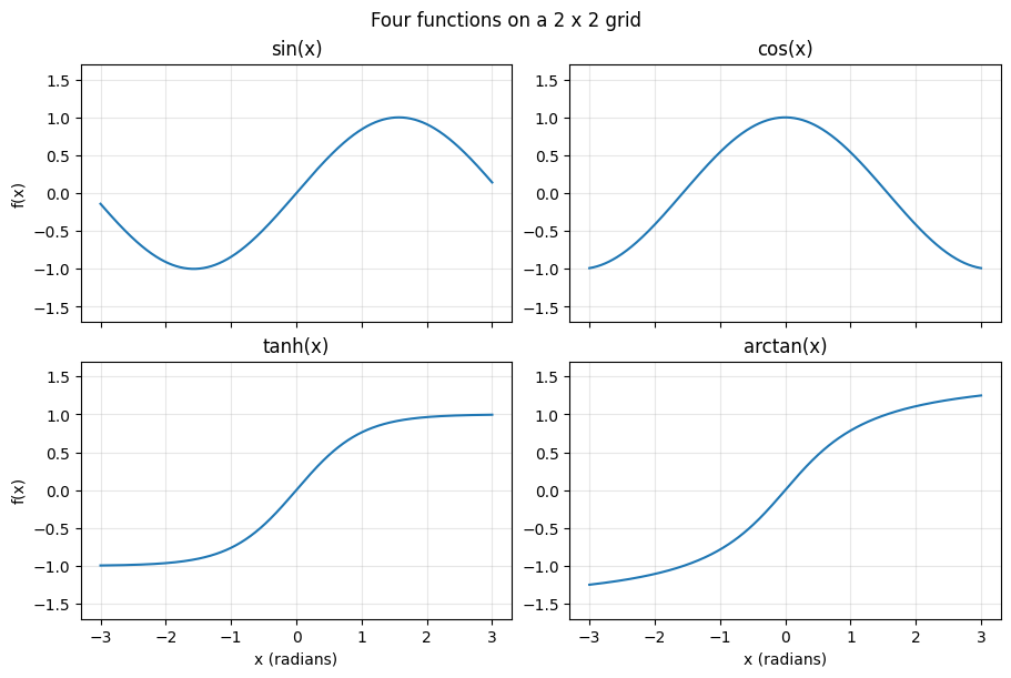
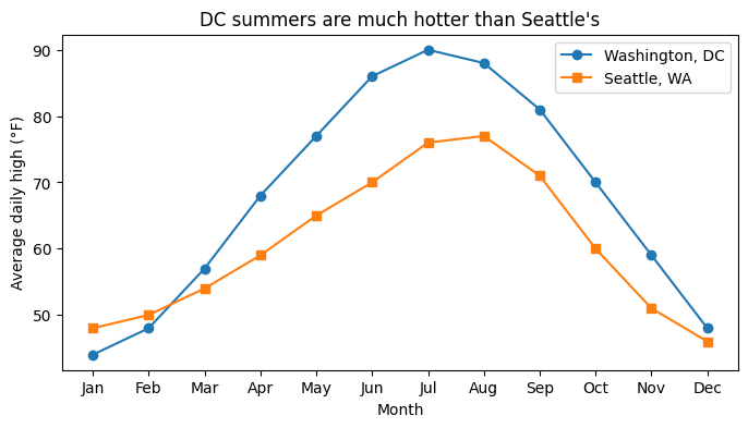
ax.plot() once per line; each call adds to the same Axeslabel= and call ax.legend() to identify them# Approximate average daily highs (°F)
seattle_high = [48, 50, 54, 59, 65, 70, 76, 77, 71, 60, 51, 46]
fig, ax = plt.subplots(figsize=(8, 4))
ax.plot(months, dc_high, marker="o", label="Washington, DC")
ax.plot(months, seattle_high, marker="s", label="Seattle, WA")
ax.set_title("DC summers are much hotter than Seattle's")
ax.set_xlabel("Month")
ax.set_ylabel("Average daily high (°F)")
ax.legend()
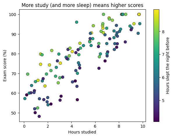
plt.show()c=) and add a colorbar to explain itn = 120
hours_studied = rng.uniform(0, 10, n)
hours_slept = rng.uniform(4, 9, n)
exam_score = np.clip(40 + 4 * hours_studied + 3 * hours_slept + rng.normal(0, 6, n), 0, 100)
fig, ax = plt.subplots(figsize=(7, 5))
points = ax.scatter(hours_studied, exam_score, c=hours_slept, cmap="viridis",
s=50, edgecolor="black", linewidth=0.5)
fig.colorbar(points, ax=ax, label="Hours slept the night before")
ax.set_title("More study (and more sleep) means higher scores")
ax.set_xlabel("Hours studied")
ax.set_ylabel("Exam score (%)")
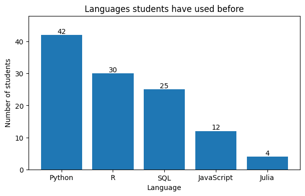
plt.show()ax.bar(categories, values) for vertical barsax.barh() for horizontal bars: better when category names are long or there are many categoriesax.bar_label() writes the value on each barlanguages = ["Python", "R", "SQL", "JavaScript", "Julia"]
n_students = [42, 30, 25, 12, 4] # illustrative survey counts
fig, ax = plt.subplots(figsize=(7, 4))
bars = ax.bar(languages, n_students, color="tab:blue")
ax.bar_label(bars)
ax.set_ylim(0, 48) # headroom so the top label fits
ax.set_title("Languages students have used before")
ax.set_xlabel("Language")
ax.set_ylabel("Number of students")
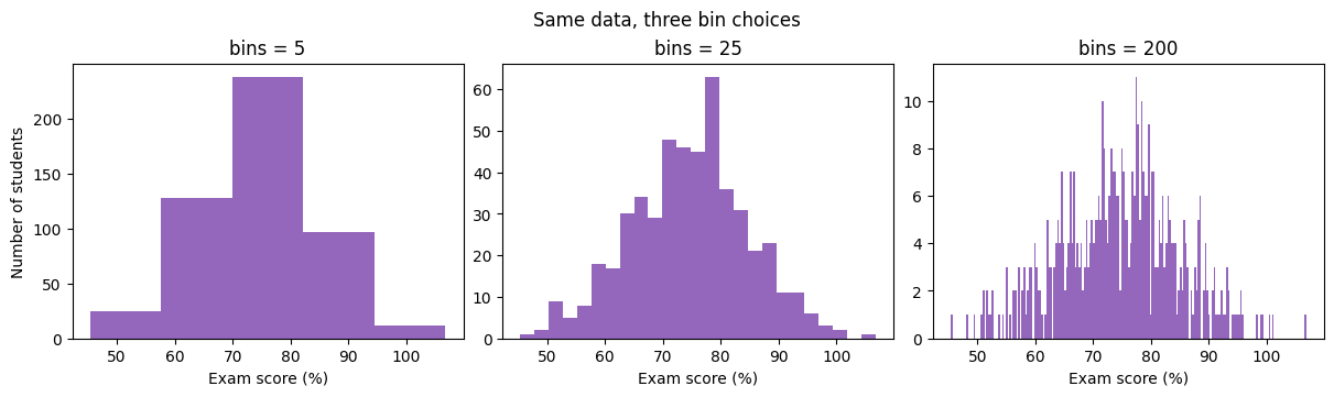
plt.show()scores = rng.normal(loc=75, scale=10, size=500)
fig, axs = plt.subplots(1, 3, figsize=(12, 3.5), layout="constrained")
for ax, bins in zip(axs, [5, 25, 200]):
ax.hist(scores, bins=bins, color="tab:purple")
ax.set_title(f"bins = {bins}")
ax.set_xlabel("Exam score (%)")
axs[0].set_ylabel("Number of students")
fig.suptitle("Same data, three bin choices")
plt.show()Every plotting method accepts keyword arguments that control its look. The most useful ones:
| Keyword | What it controls | Examples |
|---|---|---|
color |
Color | "red", "tab:blue", "#1f77b4", "C0" |
linewidth (lw) |
Line thickness (points) | 1, 2.5 |
linestyle (ls) |
Line pattern | "-", "--", ":", "-.", "none" |
marker |
Point symbol | "o", "s", "^", "x", "." |
markersize (ms) |
Marker size (plot) | 4, 10 |
s |
Marker size (scatter, it is an area) | 20, 100 |
alpha |
Transparency, 0 (invisible) to 1 (solid) | 0.3 |
label |
Name shown in the legend | "Measured" |
Ways to specify a color:
"red", "black", "gray""tab:blue", "tab:orange", "tab:green", …"#FF0000" is red ("#RRGGBB", pick codes at https://htmlcolorcodes.com)"C0", "C1", …, "C9" (the colors Matplotlib uses automatically, in order)x = np.arange(10)
fig, ax = plt.subplots(figsize=(8, 4))
ax.plot(x, x + 0, color="tab:blue", linestyle="-", marker="o", label='solid, "o"')
ax.plot(x, x + 3, color="tab:red", linestyle="--", marker="s", label='dashed, "s"')
ax.plot(x, x + 6, color="#2ca02c", linestyle=":", marker="^", label='dotted, "^"', markersize=9)
ax.plot(x, x + 9, color="black", linestyle="-.", linewidth=3, label="dash-dot, thick")
ax.set_title("Line styles, markers, and colors")
ax.legend()
plt.show()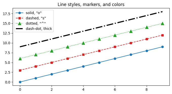
Use alpha to fix overplotting. When thousands of points pile up, a solid scatter becomes a blob. Transparency reveals where the data is dense.
big_x = rng.normal(0, 1, 5000)
big_y = big_x + rng.normal(0, 1, 5000)

fig, axs = plt.subplots(1, 2, figsize=(10, 4), sharey=True, layout="constrained")
axs[0].scatter(big_x, big_y, s=10)
axs[0].set_title("alpha = 1 (default): a blob")
axs[1].scatter(big_x, big_y, s=10, alpha=0.1)
axs[1].set_title("alpha = 0.1: density is visible")
plt.show()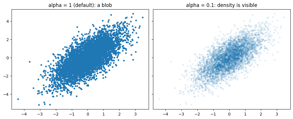
Colormaps (cmap=) map numbers to colors, used by scatter(c=...), heatmaps, and images.
"viridis" (default), "plasma", "Blues""coolwarm" or "RdBu""jet" and rainbow maps: they create fake boundaries and fail for colorblind readers| Command | What it adds |
|---|---|
ax.set_title("...") |
Title above one Axes |
fig.suptitle("...") |
Title above the whole Figure |
ax.set_xlabel("..."), ax.set_ylabel("...") |
Axis labels (always include units) |
ax.legend(loc="upper left", fontsize=12) |
Legend built from every label= |
ax.text(x, y, "...") |
Text at data coordinates (x, y) |
ax.annotate("...", xy=..., xytext=..., arrowprops=...) |
Text with an arrow pointing at a spot |
ax.axhline(y) / ax.axvline(x) |
Horizontal / vertical reference line |
Every text command accepts fontsize=, color=, and fontweight="bold".
Shortcut: ax.set(title=..., xlabel=..., ylabel=..., xlim=..., ylim=...) sets several properties in one call.
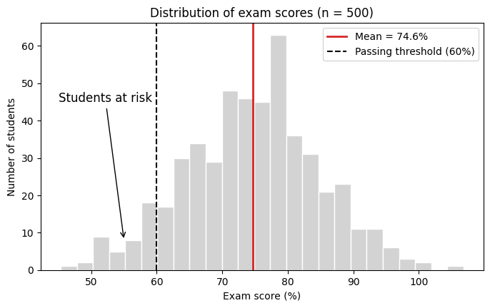
fig, ax = plt.subplots(figsize=(8, 4.5))
ax.hist(scores, bins=25, color="lightgray", edgecolor="white")

mean_score = scores.mean()
ax.axvline(mean_score, color="tab:red", linewidth=2, label=f"Mean = {mean_score:.1f}%")
ax.axvline(60, color="black", linestyle="--", label="Passing threshold (60%)")

ax.annotate("Students at risk",
            xy=(55, 8), xytext=(45, 45),
            arrowprops=dict(arrowstyle="->", color="black"),
            fontsize=12)

ax.set(title="Distribution of exam scores (n = 500)",
       xlabel="Exam score (%)",
       ylabel="Number of students")
ax.legend(loc="upper right")
plt.show()| Command | Purpose |
|---|---|
ax.set_xlim(lo, hi) / ax.set_ylim(lo, hi) |
Zoom to a range |
ax.set_xticks([...]) |
Choose where ticks go |
ax.set_xticks([...], ["a", "b", ...]) |
Choose ticks and their text labels |
ax.tick_params(labelsize=14, rotation=45) |
Tick label size / rotation |
ax.set_yscale("log") |
Logarithmic axis |
ax.grid(True, alpha=0.3) |
Light background grid |
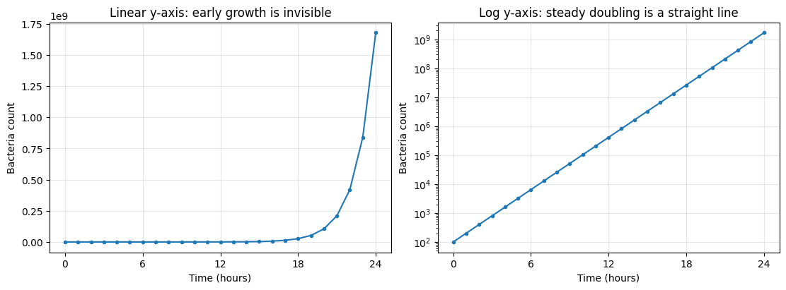
When to use a log scale: data that spans several orders of magnitude, or grows exponentially. On a log axis, exponential growth becomes a straight line.
hours = np.arange(0, 25)
bacteria = 100 * 2 ** hours              # population doubles every hour

fig, axs = plt.subplots(1, 2, figsize=(11, 4), layout="constrained")

axs[0].plot(hours, bacteria, marker=".")
axs[0].set_title("Linear y-axis: early growth is invisible")

axs[1].plot(hours, bacteria, marker=".")
axs[1].set_yscale("log")
axs[1].set_title("Log y-axis: steady doubling is a straight line")

for ax in axs:
    ax.set_xlabel("Time (hours)")
    ax.set_ylabel("Bacteria count")
    ax.set_xticks([0, 6, 12, 18, 24])
    ax.grid(True, alpha=0.3)
plt.show().png: images for slides, websites, reports (raster; set dpi=300 for sharp results).pdf / .svg: vector graphics that stay sharp at any zoom (best for papers and LaTeX)bbox_inches="tight": trims extra white space and prevents labels from being cut offplt.show(): in scripts, show() can clear the figure, giving you a blank filefig, ax = plt.subplots()
ax.plot(months, dc_high, marker="o")
ax.set(title="DC average daily high", xlabel="Month", ylabel="Temperature (°F)")
fig.savefig("dc_temps.png", dpi=300, bbox_inches="tight") # 1. save
fig.savefig("dc_temps.pdf", bbox_inches="tight")
plt.show() # 2. then show
print("Saved dc_temps.png and dc_temps.pdf to the current folder")Saved dc_temps.png and dc_temps.pdf to the current folderSame data both times: noisy measurements of a spring that slowly stops bouncing.
t = np.linspace(0, 20, 80)                               # time (s)
model = 10 * np.exp(-t / 6) * np.cos(2 * t)              # true motion (cm)
measured = model + rng.normal(0, 0.8, t.size)            # noisy sensor readings

# BEFORE: pure defaults
plt.rcdefaults()          # temporarily go back to factory defaults for a fair comparison
fig, ax = plt.subplots()
ax.plot(t, measured)
ax.plot(t, model)
plt.show()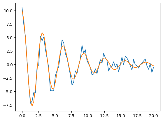
What’s wrong: no title, no labels, no units, no legend, tiny fonts, and it is unclear which line is data and which is the model.
# AFTER: every guideline applied
t_smooth = np.linspace(0, 20, 500)
model_smooth = 10 * np.exp(-t_smooth / 6) * np.cos(2 * t_smooth)
FS = 16

fig, ax = plt.subplots(figsize=(10, 5.5), layout="constrained")

ax.plot(t, measured, "o", color="tab:red", markersize=6, alpha=0.6, label="Sensor measurements")
ax.plot(t_smooth, model_smooth, color="tab:blue", linewidth=2.5, label="Damped oscillator model")
ax.plot(t_smooth,  10 * np.exp(-t_smooth / 6), color="gray", linestyle="--", linewidth=1.5,
        label="Decay envelope")
ax.plot(t_smooth, -10 * np.exp(-t_smooth / 6), color="gray", linestyle="--", linewidth=1.5)

ax.annotate("Amplitude halves every ~4 s",
            xy=(4.2, 5.0), xytext=(7, 8), fontsize=FS - 2,
            arrowprops=dict(arrowstyle="->", color="black"))

ax.set_title("A damped spring: the model matches the measurements", fontsize=FS + 4)
ax.set_xlabel("Time (s)", fontsize=FS)
ax.set_ylabel("Displacement from rest (cm)", fontsize=FS)
ax.tick_params(labelsize=FS - 2)
ax.set_xlim(0, 20)
ax.set_ylim(-11, 11)
ax.grid(alpha=0.3)
ax.legend(fontsize=FS - 2, loc="lower right")

fig.savefig("damped_spring.png", dpi=300, bbox_inches="tight")
plt.show()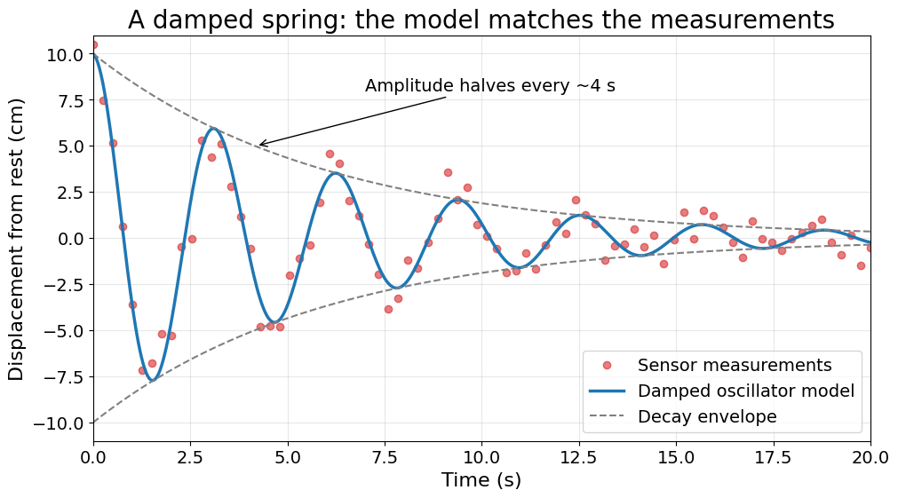
Checklist that the “after” plot satisfies: clear takeaway in the title, units on both axes, readable fonts, data and model visually distinct (markers vs. line), legend, light grid, one annotation that supports the message, nothing overlapping.