Code
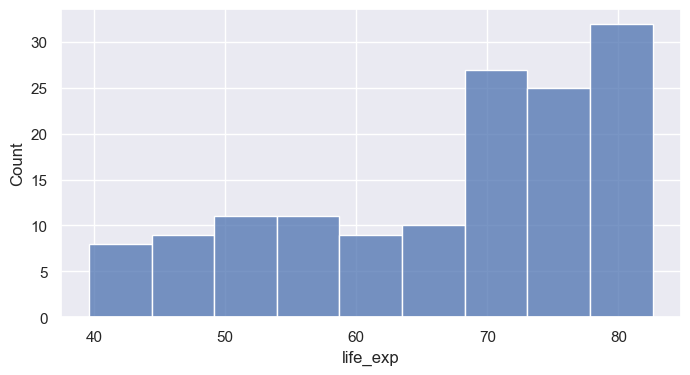
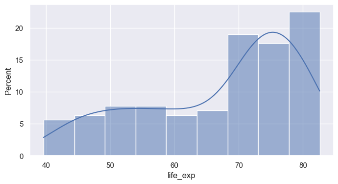
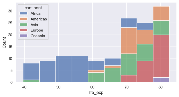
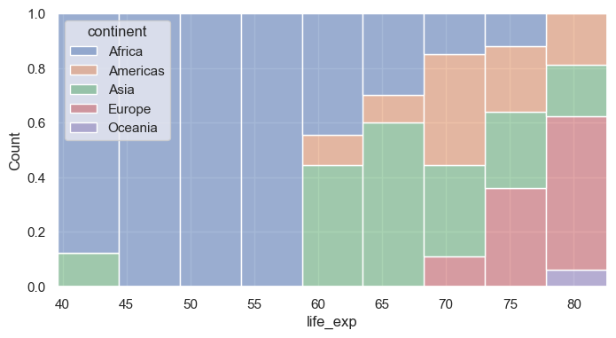
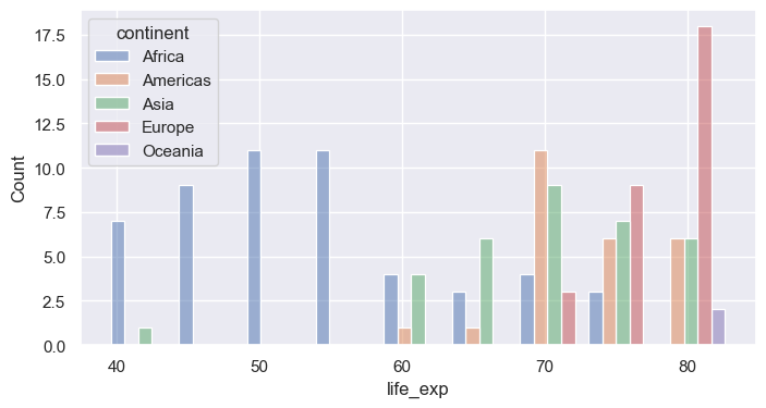
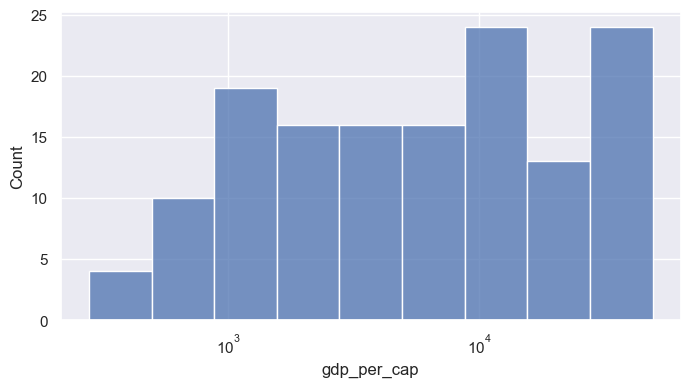
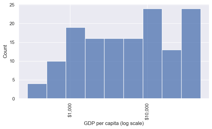
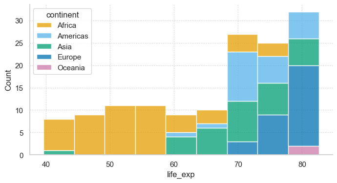
seaborn 0.13.2histplot bins one numeric variable and counts observations per binbins= sets number of bins; binwidth= sets their width (often more interpretable)stat= changes the y-axis: "count", "percent", "density", "probability"kde=True overlays a smooth density estimatehuehue= maps a categorical column to colormultiple= controls overlap: "layer" (default), "stack", "dodge", "fill"Caption: In a stacked histogram, each bar’s total height represents the total number of observations for that bin, with each color stacked on top of the previous one. For example, the blue bars at the top do not show large counts on their own—they are added above the other colors, so a short blue bar still means a small number, even if it’s high up on the plot.
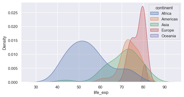
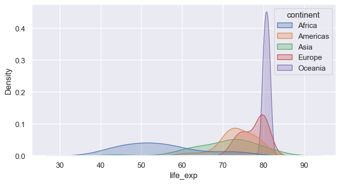
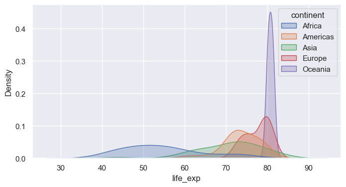
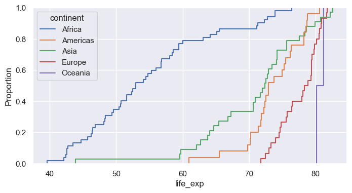
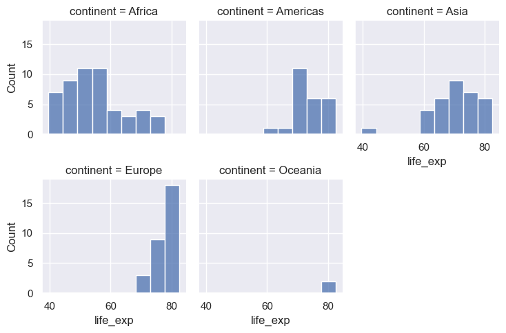
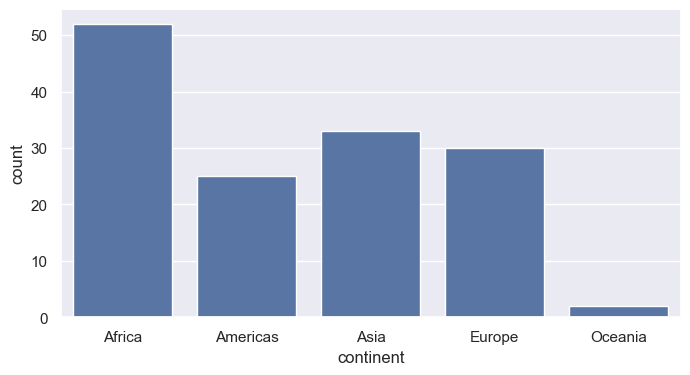
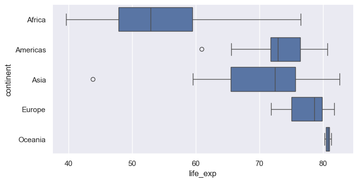
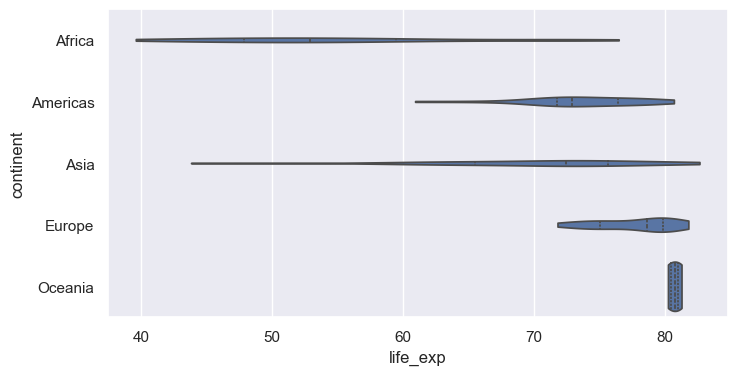
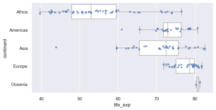
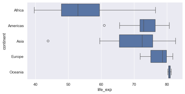
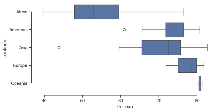
kdeplot draws a smoothed estimate of the distributionfill=True shades the area; common_norm=False normalizes each group separatelybw_adjust= controls smoothness (smaller = wigglier)log_scale=True bins on a log axis, revealing structure hidden in the raw scaleecdfplot shows the fraction of observations at or below each valuedisplotdisplot wraps histplot, kdeplot, ecdfplot (choose with kind=)col= and row= create small multiples, one panel per categorycol_wrap= wraps panels onto multiple rows; height= / aspect= size each panelcountplotx and y for horizontal boxes (often easier to read with long labels)inner="quart" draws quartile lines; inner="point" shows observationscut=0 stops the density at the data rangestripplot plots each point with random jitterswarmplot arranges points so none overlap (best for small to medium n)barplot computes a statistic per group (default: mean) with an error barestimator= changes the statistic (e.g., "median", "sum")errorbar= controls the interval: ("ci", 95), "sd", "se", or NoneAxesAxes it drew onset_title, set_xlabel, axvline, annotate, …<class 'matplotlib.axes._axes.Axes'>
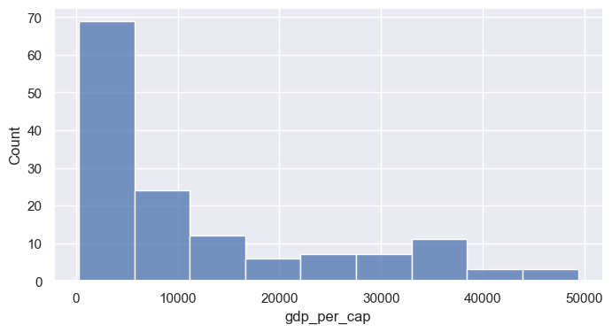
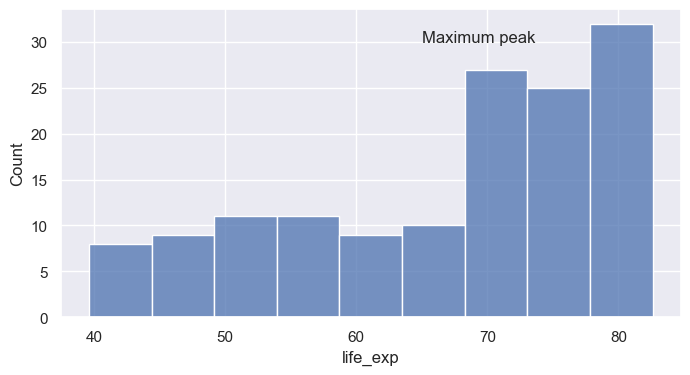
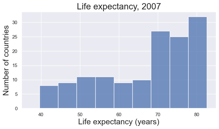
<class 'matplotlib.figure.Figure'>ax.set(...) sets many properties in one callax = sns.histplot(data=gm07, x="life_exp", binwidth=5)
# ax.set_title("A damped spring: the model matches the measurements", fontsize=12 + 4)
ax.set(title="Life expectancy, 2007", xlabel="Life expectancy (years)", ylabel="Number of countries", xlim=(35, 85))
FS=16
ax.title.set_fontsize(FS + 4)
ax.xaxis.label.set_fontsize(FS + 2)
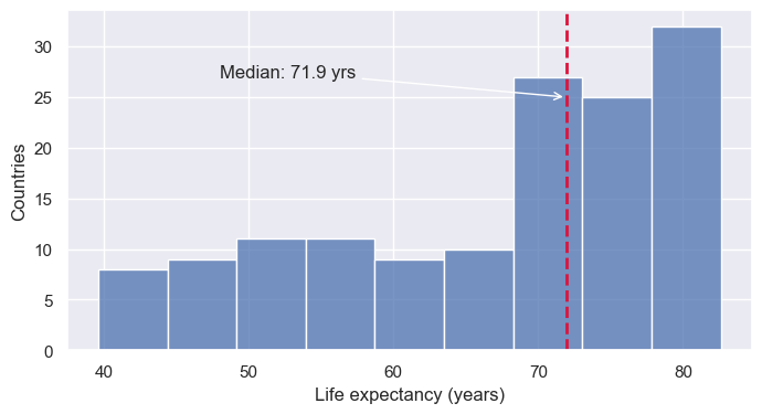
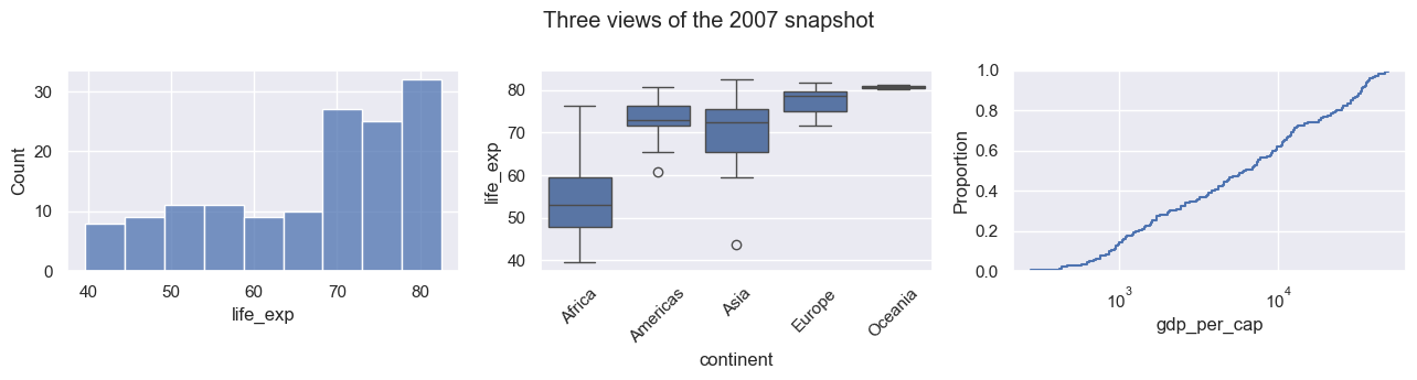
ax.yaxis.label.set_fontsize(FS + 2)axvline / axhline add vertical or horizontal reference linesax.annotate places text with an optional arrowmatplotlib.ticker formatters control tick label textax.tick_params adjusts size, rotation, and directionplt.subplots, then pass each Axes to Seaborn via ax=fig.suptitle adds an overall title; fig.tight_layout() fixes overlapsfig, axes = plt.subplots(1, 3, figsize=(13, 3.5))
sns.histplot(data=gm07, x="life_exp", ax=axes[0])
sns.boxplot(data=gm07, x="continent", y="life_exp", ax=axes[1])
sns.ecdfplot(data=gm07, x="gdp_per_cap", log_scale=True, ax=axes[2])
axes[1].tick_params(axis="x", labelrotation=45)
fig.suptitle("Three views of the 2007 snapshot")
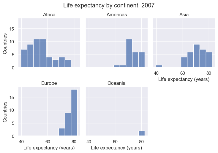
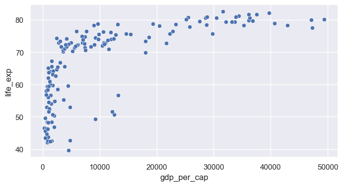
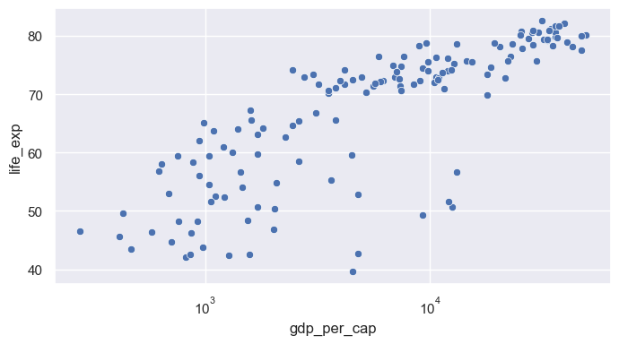
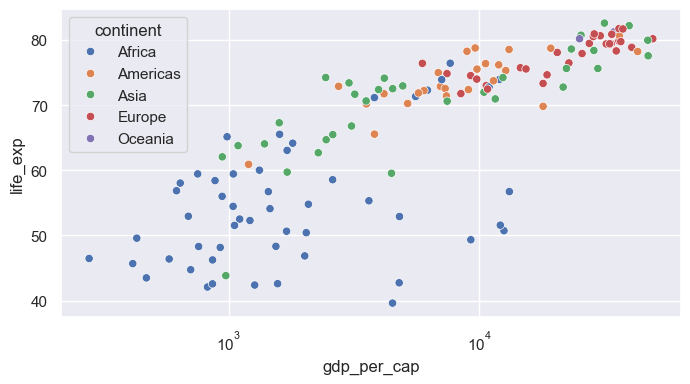
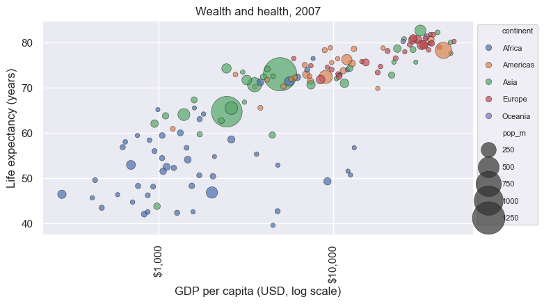
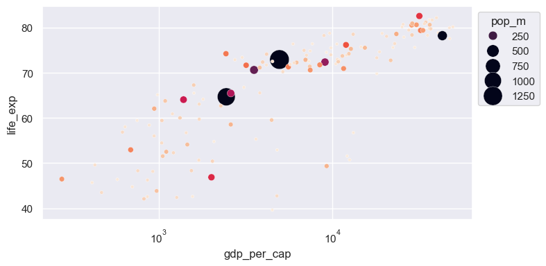
fig.tight_layout()FacetGriddisplot, catplot, relplot return a grid object, not an Axesg.figure is the matplotlib Figure; g.axes is an array of Axesg.set_axis_labels, g.set_titles, g.figure.suptitleax= to figure-level functions: they create their own figure<class 'seaborn.axisgrid.FacetGrid'>Text(0.5, 1.03, 'Life expectancy by continent, 2007')fig.savefig(...) or g.savefig(...)dpi= controls resolution; bbox_inches="tight" trims whitespace.pdf, .svg) scale cleanly in papers and slidesscatterplot maps one column to x and one to yax.set_xscale("log") (matplotlib) after plottinghuecontinent (categorical): Seaborn chooses a qualitative palette and builds the legendsize= maps a numeric column to marker area; sizes= sets the min and max sizelegend= and bbox_to_anchor move the crowded legend outside the plotax = sns.scatterplot(data=gm07, x="gdp_per_cap", y="life_exp", hue="continent", size="pop_m",
sizes=(20, 1200), alpha=0.7, edgecolor="black")
ax.set_xscale("log")
ax.xaxis.set_major_formatter(StrMethodFormatter("${x:,.0f}"))
ax.tick_params(axis="x", labelrotation=90)
ax.set(xlabel="GDP per capita (USD, log scale)", ylabel="Life expectancy (years)", title="Wealth and health, 2007")
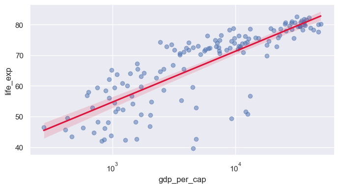
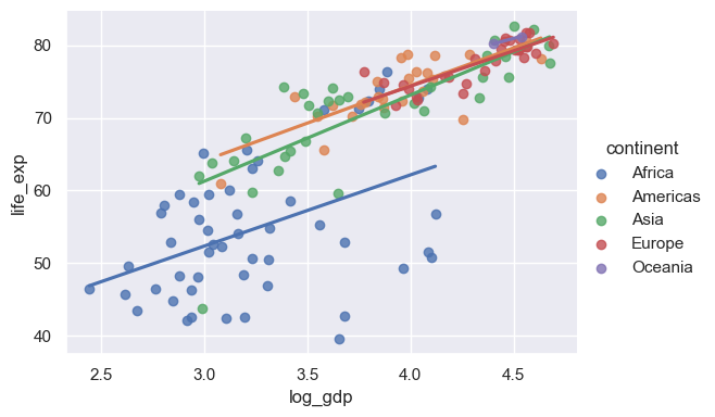
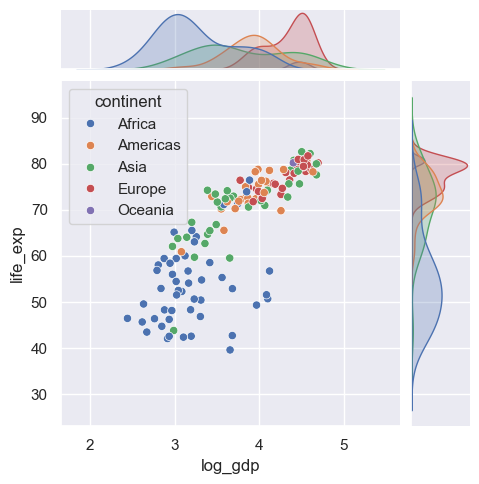
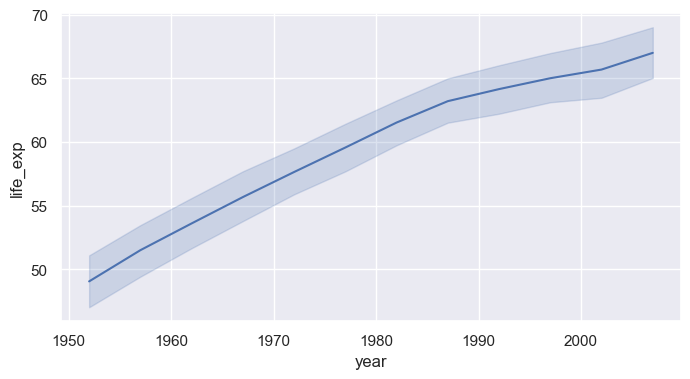
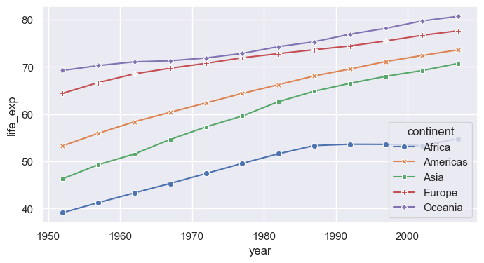
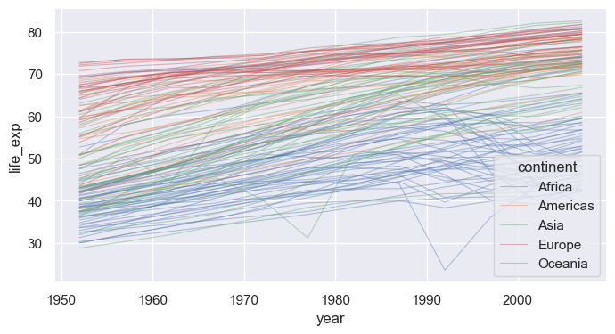
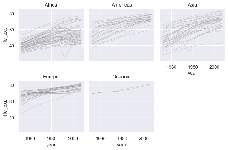
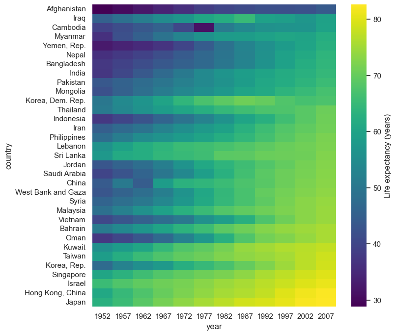
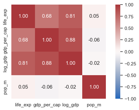
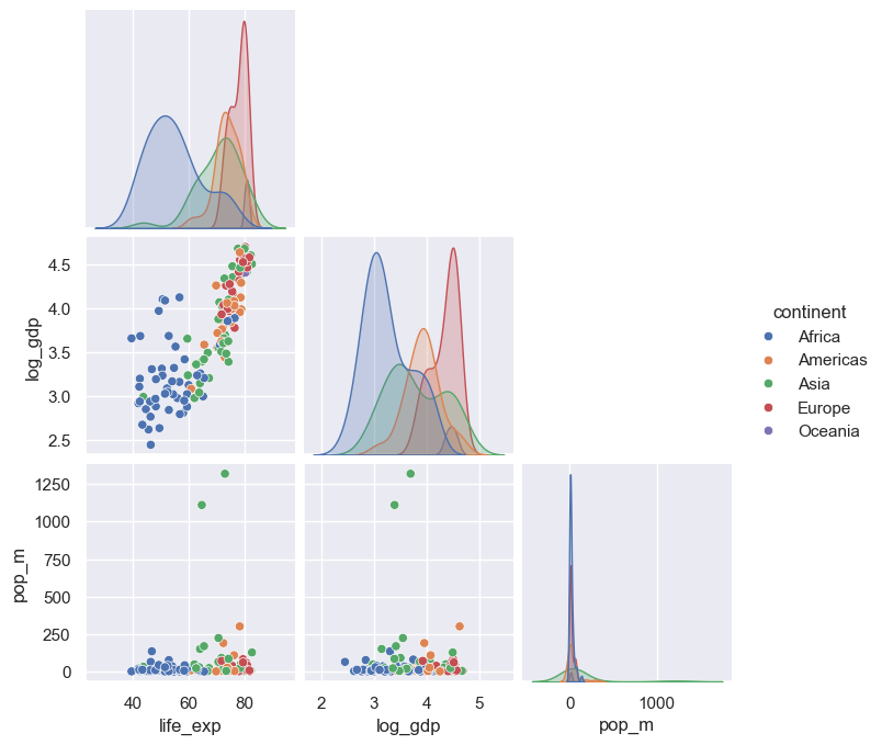
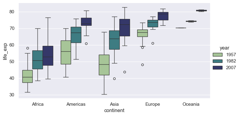
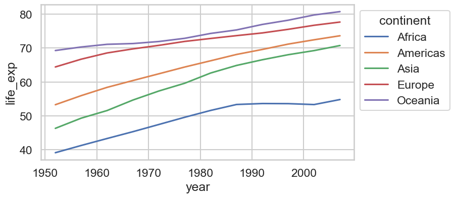
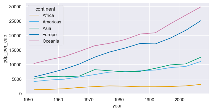
sns.move_legend(ax, "upper left", bbox_to_anchor=(1, 1), fontsize=8, labelspacing=1.3)regplotregplot draws a scatter plus a linear fit with a confidence bandlogx=True fits y against log(x); lowess=True fits a flexible smooth curvescatter_kws / line_kws pass styling to each layerlmplotregplot: supports hue, col, rowlog_gdp column)jointplotkind= options: "scatter", "kde", "hex", "reg", "hist"lineplotgm datax value, lineplot aggregates: plots the mean with a 95% CI bandhue="continent" for one aggregated line per continenterrorbar=None removes the bands; markers=True with style= marks each observation yearunitsunits= with estimator=None to draw each country separatelyrelplotscatterplot / lineplot (kind="line" or "scatter")col=, highlight a few countries on top with matplotlibheatmap displays a 2-D table as colored cellspivot rows = country, columns = year, values = life expectancycmap= sets the colormap; annot=True would print values in each celldf.corr(), then heatmap with a diverging colormap centered at 0annot=True, fmt=".2f" prints each coefficientpairplotvars= selects columns; corner=True drops the redundant upper trianglecatplotkind="box", "violin", "bar", "strip", …)x (category), y (numeric), and hue (second category)set_theme: one call for the global looksns.set_theme(style=..., context=..., palette=..., font_scale=...)darkgrid (default), whitegrid, dark, white, ticksfig = plt.figure(figsize=(16, 2.6))
for i, style in enumerate(["darkgrid", "whitegrid", "dark", "white", "ticks"]):
with sns.axes_style(style): # style applies to axes created inside the block
ax = fig.add_subplot(1, 5, i + 1)
sns.kdeplot(data=gm07, x="life_exp", fill=True, ax=ax)
ax.set(title=style, xlabel="", ylabel="", yticks=[])
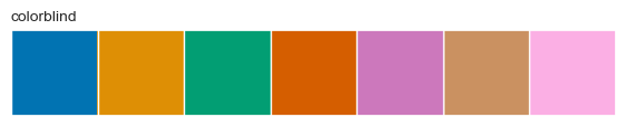
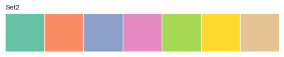
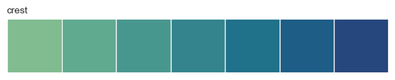
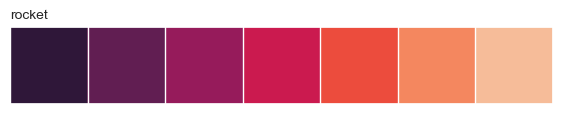
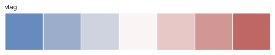
fig.tight_layout()despinewith sns.axes_style("..."): applies a style to only the plots inside the blocksns.despine() removes the top and right spines; trim=True and offset= tighten the framewhite and tickscontext= rescales fonts, lines, and markers for where the figure will be shown"paper" < "notebook" (default) < "talk" < "poster"font_scale= fine-tunes on top of the context"deep" (default), "Set2", "colorblind""viridis", "rocket", "crest", "Blues""vlag", "coolwarm", "RdBu"sns.color_palette(name, n) returns a palette; sns.palplot previews itpalette="name" on any function with huesns.set_palette("name") or sns.set_theme(palette="name")hue uses a continuous colormap; pass a sequential palettepalette={category: color} to fix colors per grouprc parametersset_theme(rc={...}) passes any matplotlib setting through Seabornplt.rcParams.keys()sns.set_theme(style="ticks", context="notebook", font_scale=1.05)
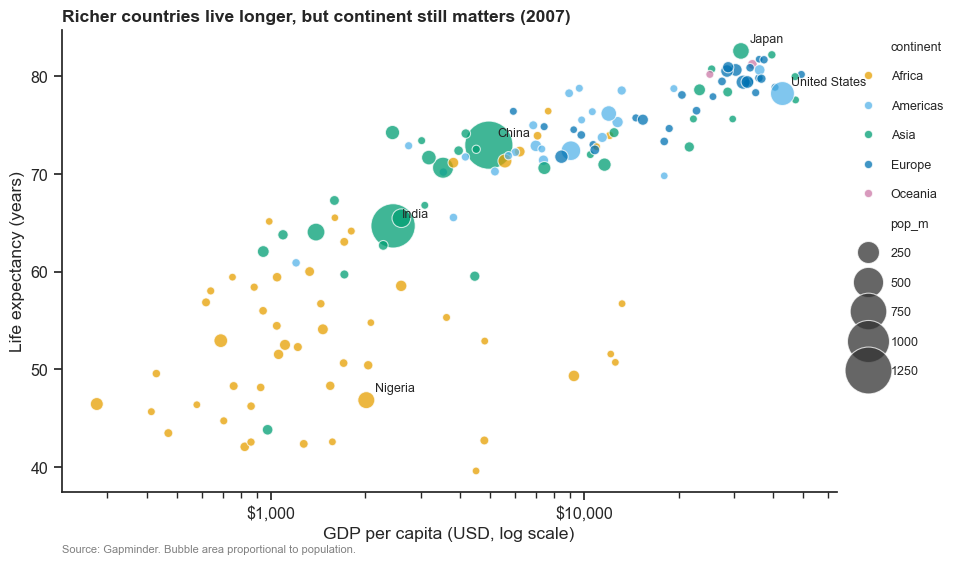
fig, ax = plt.subplots(figsize=(10, 6))
sns.scatterplot(data=gm07, x="gdp_per_cap", y="life_exp", hue="continent", size="pop_m", sizes=(30, 1200),
palette=cont_colors, alpha=0.75, edgecolor="white", linewidth=0.8, ax=ax)
ax.set_xscale("log")
ax.xaxis.set_major_formatter(StrMethodFormatter("${x:,.0f}"))
for name in ["China", "India", "United States", "Japan", "Nigeria"]:
r = gm07.loc[gm07["country"] == name].iloc[0]
ax.annotate(name, (r["gdp_per_cap"], r["life_exp"]), xytext=(6, 6), textcoords="offset points", fontsize=9)
ax.set(xlabel="GDP per capita (USD, log scale)", ylabel="Life expectancy (years)")
ax.set_title("Richer countries live longer, but continent still matters (2007)", loc="left", fontweight="bold")
ax.text(0, -0.13, "Source: Gapminder. Bubble area proportional to population.", transform=ax.transAxes, fontsize=8, color="gray")
sns.move_legend(ax, "upper left", bbox_to_anchor=(1.01, 1), frameon=False, fontsize=9, labelspacing=1.4)
sns.despine()