—; title: ‘Plotly: Client-side interactive visualization’
Overview and introduction
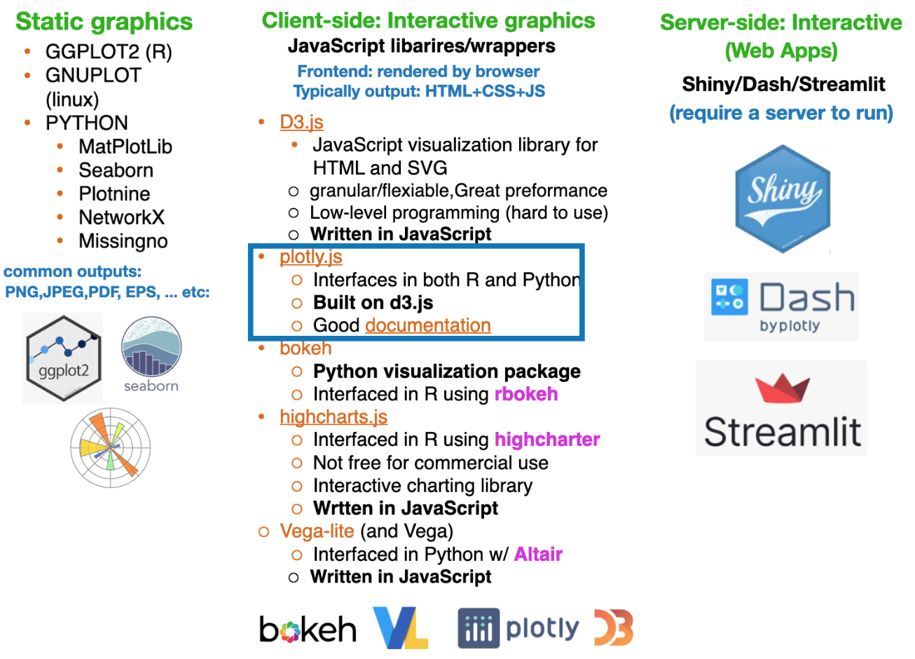
plotly.js for R and Python.Bottom line: Plotly.js leverages D3.js internally, but abstracts away its low-level complexity for end users.
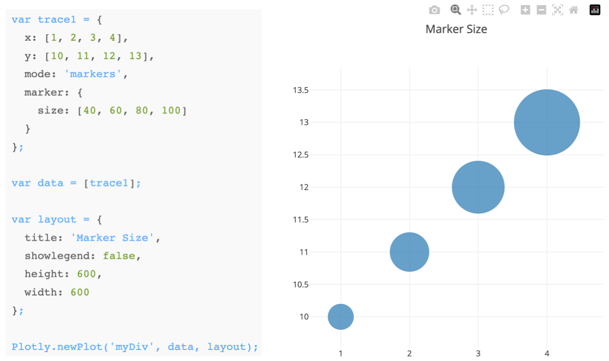
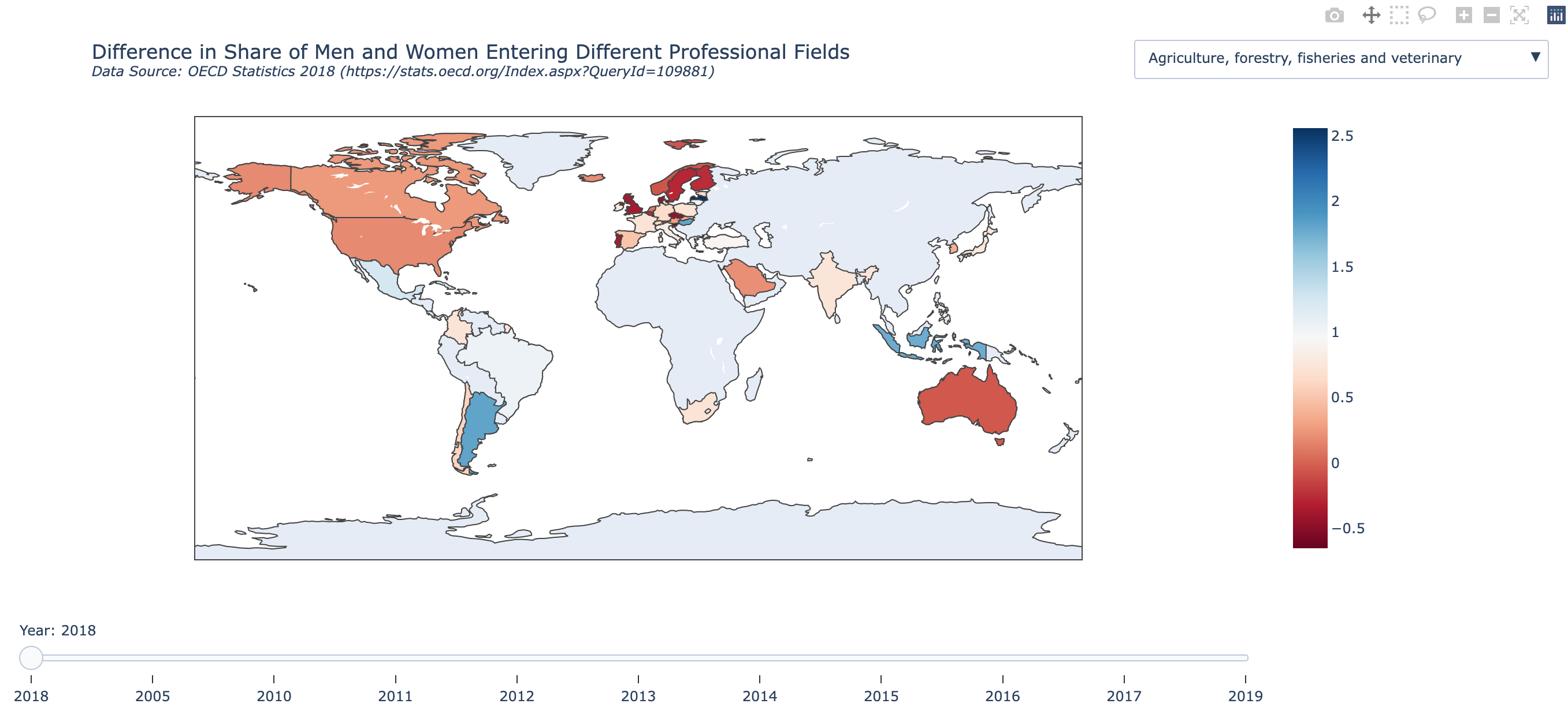
Plotly plots have interactive controls, shown in the top-right, to do the following:

Source: click here
Interactivithy introduces a new dimension of story-telling (author driven vs user driven)
These can be used for inspiration for your projects
The Pudding – A standalone data storytelling site with deeply interactive, explanatory articles on culture, sports, and social trends, built around data narratives and visual exploration. ([The Pudding][1])
FlowingData – A long-running visualization site by Nathan Yau combining analysis, charts, and narrative to help explain insights from data in engaging ways. ([Blogs Database][2])
DataJournalism.com – A central hub for data journalism practitioners and learners, featuring free resources, case studies, and links to standout projects (not a single “story,” but a repository of many). ([DataJournalism.com][3])
Interactive data storytelling projects via Flourish – While not a single traditional “website,” Flourish’s gallery showcases free, embeddable interactive visualizations (e.g., bar chart races, scrollytelling) that exemplify modern data storytelling techniques. ([Flourish][4])
Awesome Interactive Journalism (GitHub curation) – A community-maintained list linking to a broad set of free interactive journalism and data storytelling projects from around the web. ([GitHub][5])
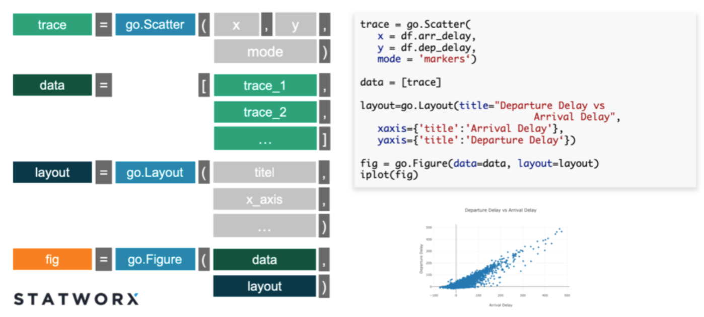
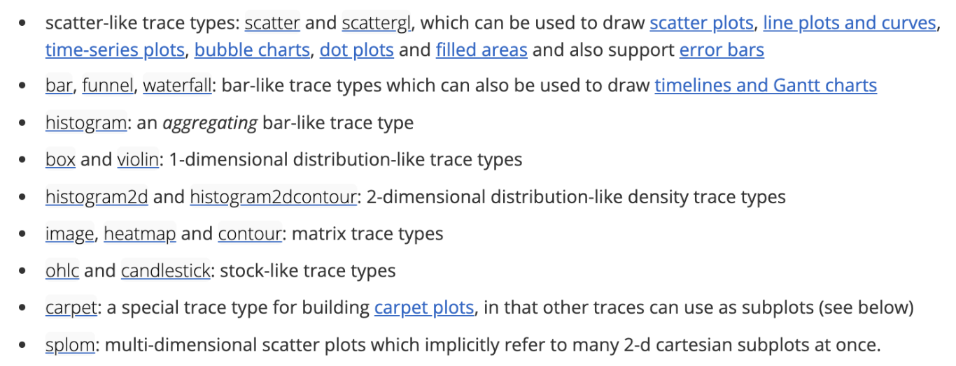
x, y, z, values).Rule of thumb: You build figures by adding traces to a figure and controlling behavior via layout.
Plotly.js in pure JavaScript form in Lab-3.1JavaScript version of Plotly, such as traces, layout, and data, are also mirrored in the Python and R wrappers that we will see later.trace type (scatter, box, , etc).
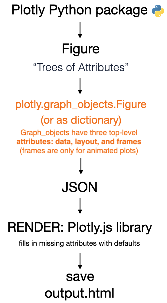
The Python (or R) wrappers create JSON files that map from python commands to the format needed by plotly.js with these fundamental components
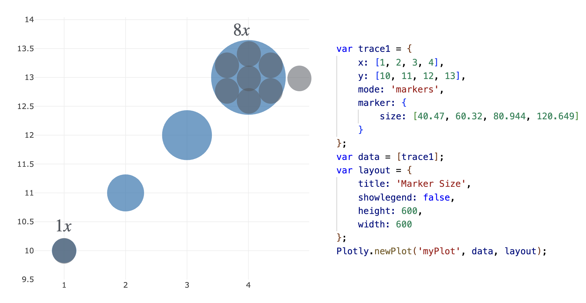
Original data encoded as marker size:

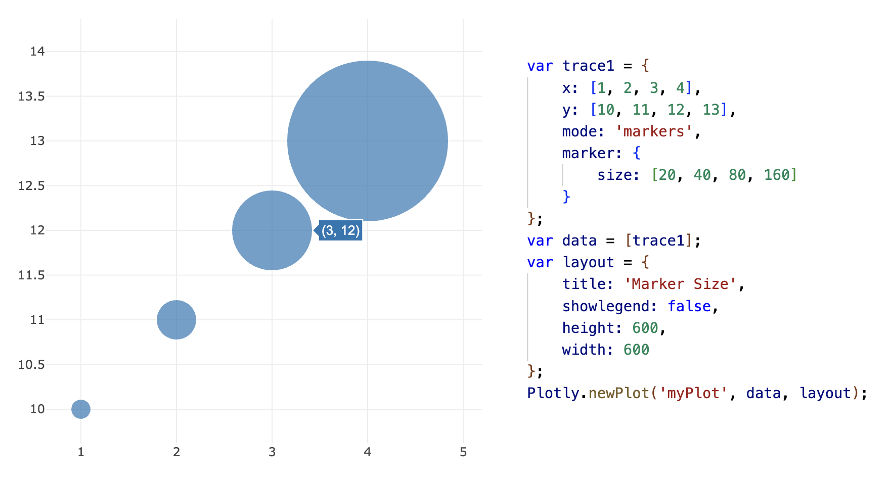
Square root transformation:
Introduction to plotly.py
Plotly figure (i.e. charts, plots, maps and diagrams)
JSON file to be rendered by plotly.js.
plotly.express module which is a set of Python functions to return completed plotly.graph_objects.Figure objects.graph_objects module which has more control, customization, and understanding of whats happening “under the hood”Plotly Express is a better starting point for plot creation, since it is powerful and easy
Plotly Express functions use graph objects internally and return a plotly.graph_object
It is good to use the graph_objects module in the following cases:
Non-standard visualizations: It is difficult to create non-standard graphs with Plotly Express, therefore graph_objects must be used
When you have a lot of customizations: If you want to make a lot of changes to most aspects of your charts, you might end up writing the same amount of code and putting in the same amount of effort, so you might consider doing it directly using the graph_objects module.
Sub-plots: Sometimes you want to have multiple charts side by side, or in a grid. If these are different charts and not facets, then it’s better to do with graph_objects.
.qmd or .rmd usually the figures will render correctly “inline” without saving the file or adding more code.ipynb sometimes the rendering can be buggy, especially in VS-code. If it doesn’t render correctly then you can do the following.
<iframe src="file_name.html" height="1000" width="1000"></iframe>Additionally, you can embed in python using the following commands, however the markdown+HTML option is recommended.
# CREATE FIGURE OBJECT
import plotly.express as px
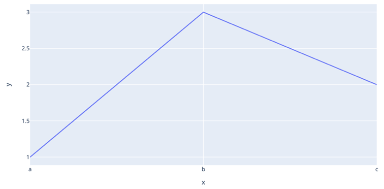
fig = px.line(x=["a","b","c"], y=[1,3,2], title="sample figure")
# SAVE TO FILES
file_name="./img/plotly-0.html"
fig.write_html(file_name)
# RE-LOAD AS AN IFRAME
from IPython.display import IFrame
IFrame(src=file_name, width=375, height=700)
.ipynbSource: click here
plotly.tools converters.fig = tls.mpl_to_plotly(mpl_fig) from import plotly.tools as tls# import warnings
# warnings.filterwarnings("ignore")
# IMPORT MODULES
import numpy as np
import matplotlib.pyplot as plt
import plotly.tools as tls
# CREATE DATA ARRAYS
x = np.linspace(-2.0 * np.pi, 2.0 * np.pi, 51)
y = np.sin(x)
# MAKE A MPL FIGURE
mpl_fig = plt.figure()
plt.plot(x, y, "ko--")
plt.xlabel("x")
plt.ylabel("sin(x)")
# plt.show()
# CONVERT USING PLOTLY
fig = tls.mpl_to_plotly(mpl_fig)
# UPDATE THEME
fig.update_layout(template="plotly_white")
fig.update_layout(width=800, height=400)
# SHOW
fig.show()
# # # SAVE AND RENDER
# file_name="./img/mpl-to-plotly.html"
# fig.write_html(file_name)
# from IPython.display import IFrame
# IFrame(src=file_name, width=900, height=500)Getting started with Plotly express
Note: Repeated package imports are intentional to make the code cells self contained
fig.update_layout()Source: click here
scatter, line, area, bar, funnel, timelinepie, sunburst, treemap, icicle, funnel_areahistogram, box, violin, strip, ecdfdensity_heatmap, density_contour, imshowscatter_3d, line_3dscatter_matrix, parallel_coordinates, parallel_categoriesscatter_mapbox, line_mapbox, choropleth_mapbox, density_mapboxscatter_geo, line_geo, choroplethscatter_polar, line_polar, bar_polarscatter_ternary, line_ternarySource: click here
Gap-minder data-setgapminder data-setShape = (1704, 7)
country continent year lifeExp pop gdpPercap iso_alpha
0 Afghanistan Asia 1952 28.801 8425333 779.445314 AFG
1 Afghanistan Asia 1957 30.332 9240934 820.853030 AFG
2 Afghanistan Asia 1962 31.997 10267083 853.100710 AFG
3 Afghanistan Asia 1967 34.020 11537966 836.197138 AFG
4 Afghanistan Asia 1972 36.088 13079460 739.981106 AFG
Tips data-setTips data-set total_bill tip sex smoker day time size
0 16.99 1.01 Female No Sun Dinner 2
1 10.34 1.66 Male No Sun Dinner 3
2 21.01 3.50 Male No Sun Dinner 3
3 23.68 3.31 Male No Sun Dinner 2
4 24.59 3.61 Female No Sun Dinner 4
.. ... ... ... ... ... ... ...
239 29.03 5.92 Male No Sat Dinner 3
240 27.18 2.00 Female Yes Sat Dinner 2
241 22.67 2.00 Male Yes Sat Dinner 2
242 17.82 1.75 Male No Sat Dinner 2
243 18.78 3.00 Female No Thur Dinner 2
[244 rows x 7 columns]
import plotly.express as px
import seaborn as sns
# GET DATA
df = sns.load_dataset("penguins")
# print(df.keys())
df = df.dropna() # drop rows with nan
# GENERATE PLOTLY FIGURE
fig = px.scatter(
data_frame=df,
x="bill_length_mm",
y="body_mass_g",
# color="body_mass_g",
color="species",
template="plotly_white", # THEME
labels={"body_mass_g": "Body mass (grams)", "bill_length_mm": "Bill length (mm)"},
title="Visualization of penguins species phenotypical clustering",
)
# MAKE POINTS LARGER AND CHANGE FONT
fig.update_traces(marker_size=14)
fig.update_layout(font={"size": 18})
# SHOW
fig.show()import plotly.express as px
import seaborn as sns
# GET DATA
df = sns.load_dataset("penguins")
# print(df.keys())
df = df.dropna() # drop rows with nan
# print(list(df["bill_length_mm"]))
# GENERATE PLOTLY FIGURE
fig = px.scatter(
x=list(df["bill_length_mm"]),
y=list(df["body_mass_g"]),
color=list(df["body_mass_g"]),
template="plotly_white", # THEME
labels={"x": "Body mass (grams)", "y": "Bill length (mm)"},
title="Visualization of penguins species phenotypical clustering",
)
# MAKE POINTS LARGER AND CHANGE FONT
fig.update_traces(marker_size=14)
fig.update_layout(font={"size": 18}, height=450)
# SHOW
fig.show()As usual with most packages, the default styling is quite bad
Even just a few minor tweaks brings the graph much closer to publication quality
# Import necessary libraries
import plotly.express as px
import seaborn as sns
# Load the penguins dataset from seaborn
df = sns.load_dataset("penguins")
# Create a scatter matrix (pair plot) using selected dimensions (columns)
fig = px.scatter_matrix(
df,
dimensions=[
"bill_length_mm", # Penguin bill length in mm
"bill_depth_mm", # Penguin bill depth in mm
"flipper_length_mm", # Penguin flipper length in mm
"body_mass_g", # Penguin body mass in grams
],
color="species", # Differentiate points by species with colors
width=900, # Set plot width
height=900, # Set plot height
labels={
"bill_length_mm": "Bill length (mm)",
"bill_depth_mm": "Bill depth (mm)",
"flipper_length_mm": "Flipper length (mm)",
"body_mass_g": "Body mass (g)",
}, # Custom axis labels
)
# Hide the diagonal (histograms) in the scatter matrix
fig.update_traces(diagonal_visible=False)
# Set a clean white template for the plot background and grid
fig.update_layout(template="plotly_white")
# Display the figure
fig.show()Plotly-expressimport plotly.express as px
# EXAMPLE-1
df = px.data.gapminder()
fig = px.line(
df,
x="year",
y="lifeExp",
color="continent",
line_group="country",
hover_name="country",
height=500,
width=1000,
template="presentation",
labels={"lifeExp": "Life expectancy (years)", "year": "Time (years)"},
)
fig.update_layout(showlegend=True)
fig.show()Plotly-expressimport plotly.express as px
tips = px.data.tips()
# print(tips)
# DEFAULT
fig = px.bar(
tips,
x="day",
y="total_bill",
width=500,
height=500,
labels={
"day": "Day",
"total_bill": "Total bill",
},
)
fig.show()
# ADD A GROUPING VARIABLE
fig = px.bar(
tips,
x="day",
barmode="group",
y="total_bill",
color="smoker",
category_orders={"day": ["Thur", "Fri", "Sat", "Sun"]},
width=500,
height=500,
labels={"day": "Day", "total_bill": "Total bill"},
)
fig.show()# ADD FACETING GROUPING VARIABLE
fig = px.bar(
tips,
x="day",
y="total_bill",
color="smoker",
barmode="group",
facet_col="sex",
category_orders={
"day": ["Thur", "Fri", "Sat", "Sun"],
"sex": ["Male", "Female"],
"smoker": ["Yes", "No"],
},
labels={
"day": "Day",
"total_bill": "Total bill",
"smoker": "Smoker",
"sex": "Sex",
},
width=1000,
height=400,
)
fig.show()graph objects, however you can have a similar effect with Quarto using the following in the code cell#| column: screen-inset-shaded
#| layout-nrow: 1
import plotly.express as px
import seaborn as sns
tips = px.data.tips()
# print(tips)
w = 325
h = w
# HISTOGRAM, NORMALIZED TO HAVE AREA 1
fig = px.histogram(
tips,
x="total_bill",
nbins=20,
histnorm="probability density",
color_discrete_sequence=["indianred"],
labels={"total_bill": "Total bill"},
width=w,
height=h,
)
fig.show()
# GROUPED HISTOGRAM
fig = px.histogram(
tips,
x="total_bill",
color="sex",
histnorm="probability density",
labels={"total_bill": "Total bill"},
width=w,
height=h,
)
fig.show()
# THE HISTOGRAM, APPLIED TO A CATEGORICAL VARIABLE,
# PRODUCES A FREQUENCY BAR PLOT
fig = px.histogram(
tips,
x="day",
category_orders={"day": ["Thur", "Fri", "Sat", "Sun"]},
width=w,
height=h,
)
# ORDER BY VALUE
fig.update_xaxes(categoryorder="total ascending")
fig.show()
# Bar plots of values of one variable grouped by categories
# of another
fig = (
px.histogram(tips, x="day", y="tip", histfunc="avg", width=400, height=400)
.update_xaxes(categoryorder="total ascending")
.update_layout(
yaxis_tickformat="$",
width=w,
height=h,
)
)
fig.show()violin plot displays the distribution of a continuous variable through a kernel density plot, mirrored and joined along a central axis, and can also include box plots or individual points.strip plot displays the distribution of a continuous variable as a sequence of points along a categorical axis, often with jitter or adjustment to minimize overlapping, and can also display multiple groups side by side or stacked.import plotly.express as px
import seaborn as sns
tips = px.data.tips()
# print(tips)
w = 350
h = w
# BOXPLOT
fig = px.box(
tips,
x="day",
y="total_bill",
labels={"total_bill": "Total bill"},
width=w,
height=h,
)
fig.show()
# VIOLIN PLOT
fig = px.violin(
tips,
x="day",
y="total_bill",
labels={"total_bill": "Total bill"},
width=w,
height=h,
)
fig.show()
# STRIP PLOT
fig = px.strip(
tips,
x="day",
y="total_bill",
labels={"total_bill": "Total bill"},
width=w,
height=h,
)
fig.show()A marginal plot, controlled with marginal_x and marginal_y, displays two variables along the x and y axes, with individual distributions on the margins.
Many of the Plotly graphs allow the addition of marginal plots, e.g. here we show a density_heatmap instead of a scatter plot
import plotly.express as px
import seaborn as sns
tips = px.data.tips()
# print(tips)
fig = px.density_heatmap(
tips,
x="total_bill",
y="tip",
marginal_x="histogram",
marginal_y="histogram",
color_continuous_scale=px.colors.sequential.Viridis,
nbinsx=50,
nbinsy=50,
labels={"total_bill": "Total bill", "tip": "Tip"},
title="Joint distribution of tip and total bill",
width=500,
height=500,
)
fig.show()import plotly.express as px
import seaborn as sns
tips = px.data.tips()
# print(tips)
# # GROUPED HISTOGRAM
fig = px.histogram(
tips,
x="total_bill",
color="sex",
facet_col="day",
nbins=10,
marginal="rug", # or 'rug' or 'violin'
# histnorm="probability density",
labels={"total_bill": "Total bill"},
width=1000,
height=600,
)
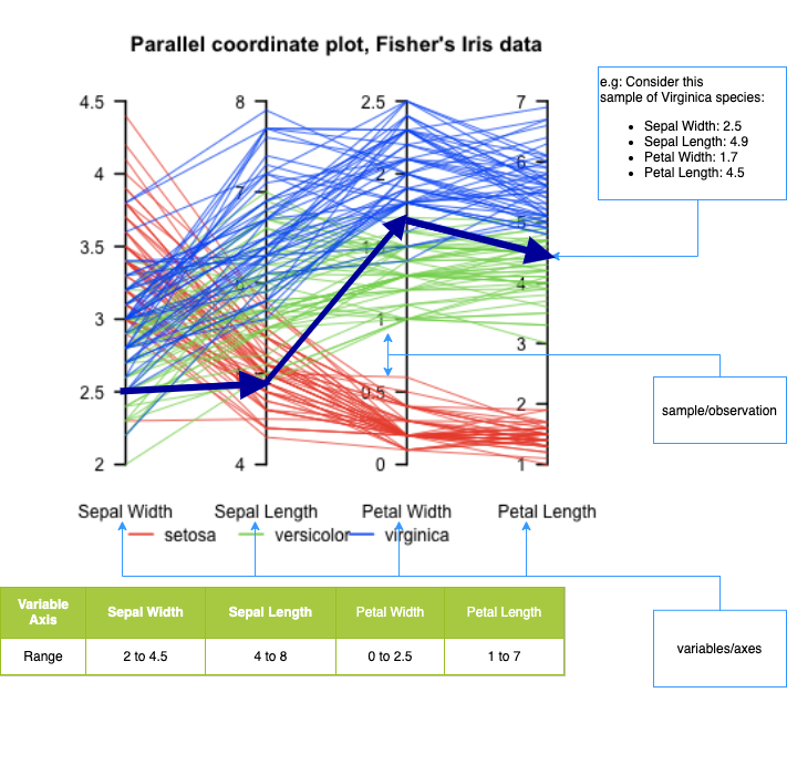
fig.show()What it is:: A visualization for multivariate data where each variable is a parallel axis, and each observation is drawn as a polyline across axes.
What it’s good for:
How to read it:
Strengths:
Limitations:
Typical use cases:
Here’s a useful example of a Parallel Coordinates plot, showing multivariate structure in the well-known Iris dataset — where different species form distinguishable patterns across four features (sepal/petal width/length):
px.parallel_coordinates()import plotly.express as px
import seaborn as sns
df = sns.load_dataset("penguins")
df = df.dropna() # drop rows with nan
print(df)
df["species"] = df.species.astype("category")
df["species_id"] = df.species.cat.codes
px.parallel_coordinates(
df,
color="species_id",
color_continuous_scale=px.colors.diverging.Tealrose,
height=300,
width=1000,
labels={"bill_length_mm": "Bill length (mm)"},
) species island bill_length_mm bill_depth_mm flipper_length_mm \
0 Adelie Torgersen 39.1 18.7 181.0
1 Adelie Torgersen 39.5 17.4 186.0
2 Adelie Torgersen 40.3 18.0 195.0
4 Adelie Torgersen 36.7 19.3 193.0
5 Adelie Torgersen 39.3 20.6 190.0
.. ... ... ... ... ...
338 Gentoo Biscoe 47.2 13.7 214.0
340 Gentoo Biscoe 46.8 14.3 215.0
341 Gentoo Biscoe 50.4 15.7 222.0
342 Gentoo Biscoe 45.2 14.8 212.0
343 Gentoo Biscoe 49.9 16.1 213.0
body_mass_g sex
0 3750.0 Male
1 3800.0 Female
2 3250.0 Female
4 3450.0 Female
5 3650.0 Male
.. ... ...
338 4925.0 Female
340 4850.0 Female
341 5750.0 Male
342 5200.0 Female
343 5400.0 Male
[333 rows x 7 columns]
px.treemap() functionimport plotly.express as px
import numpy as np
# There is no `mpg` dataset in plotly.express.data.
# We'll use the seaborn 'mpg' dataset for this example instead:
import seaborn as sns
df = sns.load_dataset("mpg").dropna()
# We'll nest the data by origin and manufacturer, and size by count (since there's no obvious "size" variable)
df["all"] = "all_cars"
# The 'mpg' dataset does not have a 'manufacturer' column; let's extract manufacturer from the 'name' (it's before the first space)
df["manufacturer"] = df["name"].apply(lambda x: x.split()[0])
mpg_counts = df.groupby(["all", "origin", "manufacturer"], as_index=False).size()
mpg_avg_mpg = df.groupby(["all", "origin", "manufacturer"], as_index=False)["mpg"].mean()
df_treemap = mpg_counts.merge(mpg_avg_mpg, on=["all", "origin", "manufacturer"], how="left")
fig = px.treemap(
df_treemap,
path=["all", "origin", "manufacturer"], # hierarchical path
values="size", # size (number of cars)
color="mpg", # average mpg by group
hover_data={"size":True, "mpg":":.1f"},
color_continuous_scale="RdBu",
color_continuous_midpoint=np.average(df["mpg"]),
height=450
)
fig.show()Unable to display output for mime type(s): application/vnd.plotly.v1+json
px.scatter_3d# SOURCE: https://towardsdatascience.com/cheat-codes-to-better-
# visualisations-with-plotly-express-21caece3db01
import plotly.express as px
import seaborn as sns
# GET DATA
election = px.data.election()
# GENERATE FIGURE
fig = px.scatter_3d(
election, # dataframe
x="Joly", # x-values column
y="Coderre", # y-values column
z="Bergeron", # z-values column
color="winner", # column shown by color
width=900,
height=600,
hover_name="district", # hover title
symbol="result", # column shown by shape
color_discrete_map={"Joly": "blue", "Bergeron": "green", "Coderre": "red"},
)
# specific colors for x,y,z values )
fig.show()Plotly Express automatically applies a square-root scaling to bubble sizes.
Specifically:
size= in functions like px.scatter, Plotly Express maps the data values to marker area, not radius.This is intentional and aligns with visualization best practices, since humans perceive area, not radius.
If you want direct control, you can:
marker.size and marker.sizeref.Key takeaway: Plotly Express does the perceptually correct thing by default for bubble plots.
Unable to display output for mime type(s): application/vnd.plotly.v1+json
# https://plotly.com/python/templates/
import plotly.express as px
df = px.data.gapminder()
df_2007 = df.query("year==2007")
k = 0
for template in [
"plotly",
"plotly_white",
"plotly_dark",
"ggplot2",
"seaborn",
"none",
"simple_white",
]:
fig = px.scatter(
df_2007,
x="gdpPercap",
y="lifeExp",
size=df_2007["pop"],
color="continent",
log_x=True,
size_max=60,
template=template,
title="Gapminder 2007: '%s' theme" % template,
)
file_name = "./img/plotly-theme-" + str(k) + ".html"
# print(file_name)
fig.write_html(file_name)
fig.show()
k += 1
# from IPython.display import IFrame
# IFrame(src=file_name, width=1000, height=500)facet_col and facet_col_wrap commandsplotly.goimport plotly.express as px
# import seaborn as sns
gap = px.data.gapminder()
fig = px.line(
data_frame=gap,
x="year",
y="lifeExp",
color="continent",
facet_col="continent",
# line_group="country",
facet_col_wrap=3, # << facet_col is the key
labels={"lifeExp": "Life expectancy"}, # , "year" : 'Time (years)'},
template="plotly_white",
width=1000,
height=1000,
).update_layout(showlegend=False)
fig.show()import plotly.express as px
import seaborn as sns
df = sns.load_dataset("penguins")
df = df.dropna() # drop rows with nan
fig = px.scatter(
data_frame=df,
x="bill_length_mm",
y="body_mass_g",
size=df["flipper_length_mm"],
color="species",
template="plotly_white",
labels={
"bill_length_mm": "Bill length (mm)",
"body_mass_g": "Body mass (g)",
"species": "Species",
},
title="Palmer Penguins",
)
# UPDATE TOOL TIP
fig.update_traces(
customdata=df,
hovertemplate="Island: %{customdata[1]} <br>Sex: %{customdata[6]}",
)
fig.show()Plotly provides a range of tools that makes adding animations to visualizations easy.
Choropleths in more detail during the Geo-spatial module.population density, then regions with higher density would be shaded darker than regions with lower population density.Plotly can internally create the map using location tags for countries, such as USA.
import plotly.express as px
import seaborn as sns
# SOURCE: https://towardsdatascience.com/cheat-codes-to-better-
# visualisations-with-plotly-express-21caece3db01
gapminder = px.data.gapminder()
fig = px.choropleth(
gapminder, # dataframe
locations="iso_alpha", # location code
color="lifeExp", # column shown by color
hover_name="country", # hover info title
animation_frame="year", # column animated
range_color=[20, 80], # color range
)
fig.show()Graph objects
Note: Graph objects are covered heavily in the lab, so we only introduce the fundamentals here
Plotly express is generally easy and straight-forward.plotly graph objects and things can get quite involved.Plotly express, however combining them with plotly graph objects is non-trivial. Figure as containerScatter, Bar, Heatmap, etc.)add_trace, update_traces, update_layoutScattergl, etc.)Plotly figures are represented as hierarchical trees, with Graph_objects being the root note, and child-nodes called attributes.data, layout, and frames (frames are only needed for animated plots)
JavaScript mentioned earlier.trace represents a set of related graphical marks in a figure.type attribute which defines the other allowable attributes.scatter, bar, pie, surface, choropleth etc)Sources: figure structure Graph objects
For more click here!

Figure({
'data': [{'hovertemplate': 'x=%{x}<br>y=%{y}<extra></extra>',
'legendgroup': '',
'line': {'color': '#636efa', 'dash': 'solid'},
'marker': {'symbol': 'circle'},
'mode': 'lines',
'name': '',
'orientation': 'v',
'showlegend': False,
'type': 'scatter',
'x': array(['a', 'b', 'c'], dtype=object),
'xaxis': 'x',
'y': {'bdata': 'AQMC', 'dtype': 'i1'},
'yaxis': 'y'}],
'layout': {'legend': {'tracegroupgap': 0},
'template': '...',
'title': {'text': 'sample figure'},
'xaxis': {'anchor': 'y', 'domain': [0.0, 1.0], 'title': {'text': 'x'}},
'yaxis': {'anchor': 'x', 'domain': [0.0, 1.0], 'title': {'text': 'y'}}}
})
(1) Initialize the figure(2) Add one or more traces(3) customize the layoutimport plotly.express as px
import plotly.graph_objects as go
# DATAFRAME
df = px.data.gapminder()
# INITIALIZE GRAPH OBJECT
fig = go.Figure()
# ADD TRACES FOR THE DATA-FRAME
fig.add_trace(
go.Scatter(
x=df["gdpPercap"],
y=df["lifeExp"],
mode="markers",
# Note: marker expects a dictionary, so use {} not dict()
marker={
"size": 50 * (df["pop"] / df["pop"].max()) ** 0.5,
"color": df["pop"],
"showscale": True,
"colorscale": "Viridis",
"symbol": "circle",
},
opacity=1.0,
)
)
# SET THEME, AXIS LABELS, AND LOG SCALE
fig.update_layout(
template="plotly_white",
xaxis_title="National GDP (per capita)",
yaxis_title="Life expectancy (years)",
title="Country comparison: color & size = population",
height=400,
width=800,
)
fig.update_xaxes(type="log")
fig.show()
With plotly.graph_objects we can finally combine figures in a subplot! source
from plotly.subplots import make_subplots
import plotly.graph_objects as go
fig = make_subplots(rows=1, cols=2)
fig.add_trace(
go.Scatter(x=[1, 2, 3], y=[4, 5, 6]),
row=1, col=1
)
fig.add_trace(
go.Scatter(x=[20, 30, 40], y=[50, 60, 70]),
row=1, col=2
)
fig.update_layout(height=500, width=700, title_text="Side By Side Subplots")
fig.show()Here we show a 2 x 2 subplot grid with each subplot populated with a single scatter trace.
import plotly.graph_objects as go
from plotly.subplots import make_subplots
fig = make_subplots(rows=2, cols=2, start_cell="bottom-left")
fig.add_trace(go.Scatter(x=[1, 2, 3], y=[4, 5, 6]),
row=1, col=1)
fig.add_trace(go.Scatter(x=[20, 30, 40], y=[50, 60, 70]),
row=1, col=2)
fig.add_trace(go.Scatter(x=[300, 400, 500], y=[600, 700, 800]),
row=2, col=1)
fig.add_trace(go.Scatter(x=[4000, 5000, 6000], y=[7000, 8000, 9000]),
row=2, col=2)
fig.show()What they are: Layout-level UI controls (layout.sliders) made of discrete steps that update figure state.
What they do: Select among predefined states by updating trace visibility, data, or layout — no dynamic computation.
Common pattern (masking):
visible masks to show the active trace(s)Alternative pattern (animations):
Rule of thumb:
SVG Traces
WebGL Traces
Rule of thumb: Use SVG for publication-quality visuals and WebGL when performance with large data matters.
You switch by choosing the trace type (not a global flag).
Other common WebGL variants:
go.Pointcloudgo.HeatmapglKey point: SVG vs WebGL is a trace-level decision—use WebGL (*gl traces) when performance matters, SVG otherwise.
from plotly.subplots import make_subplots
import plotly.graph_objects as go
fig = go.Figure()
N=100000
x=np.random.randn(N)
y=2*x+np.random.randn(N)
fig.add_trace(go.Scattergl(x=x, y=y, mode="markers"))
# fig.add_trace(go.Scatter(x=x, y=y, mode="markers"))
fig.update_layout(height=500, width=700, title_text="Side By Side Subplots")
fig.show()plotly-express and graph-objects, which can get you started on almost any task. Optional: additional content
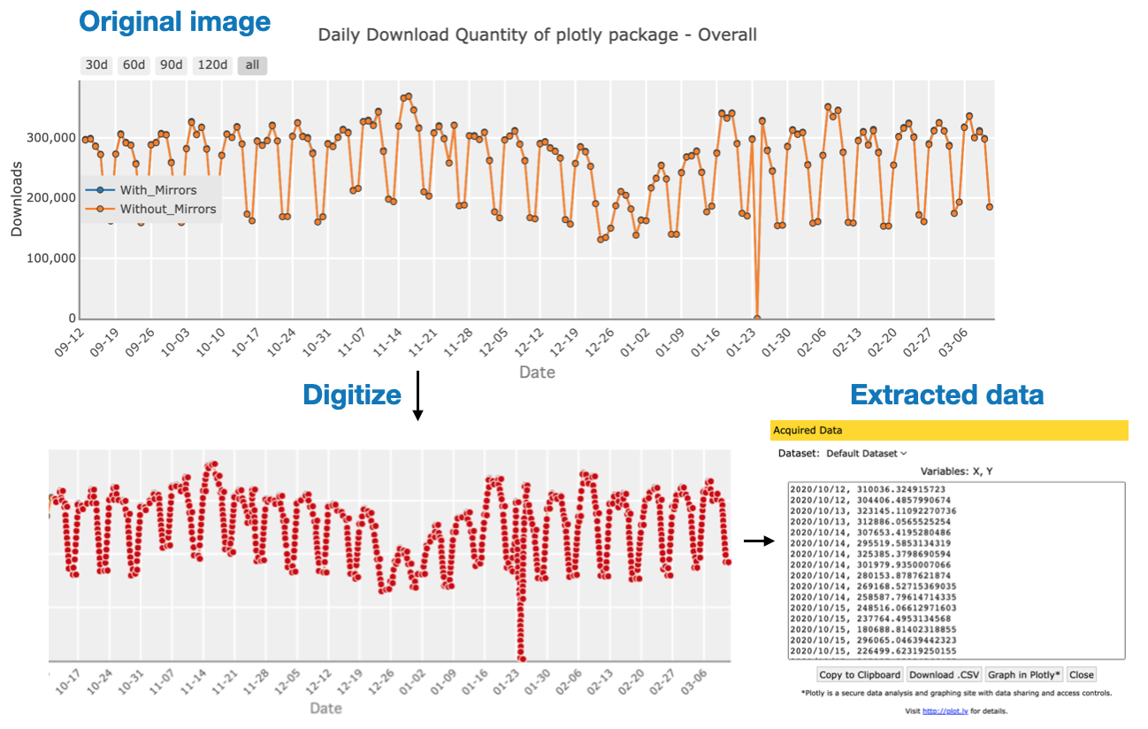
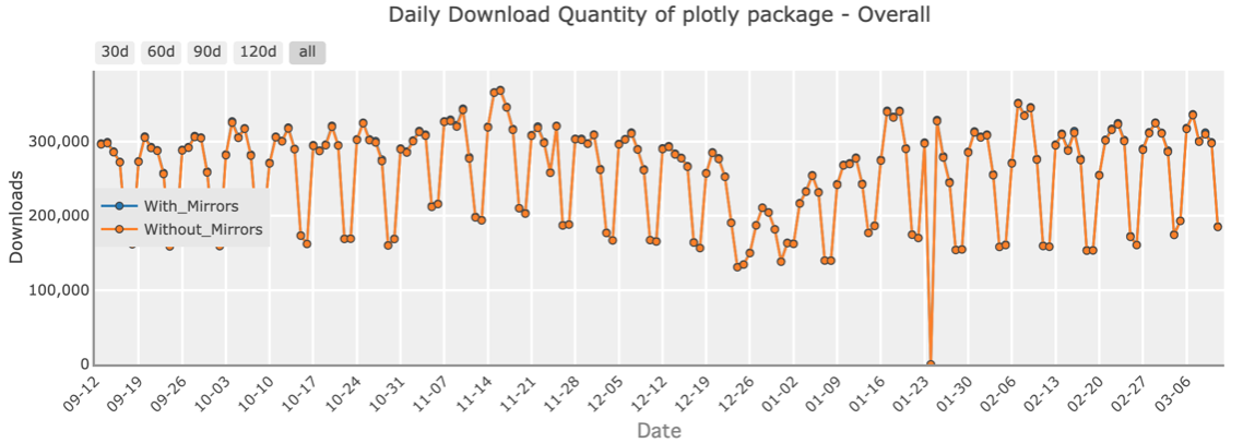
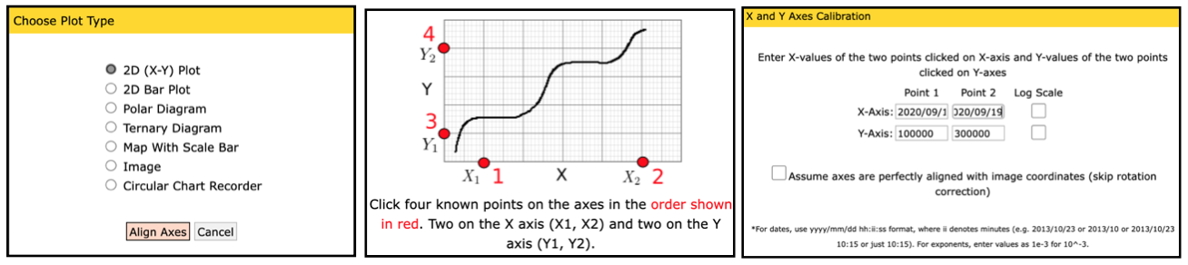
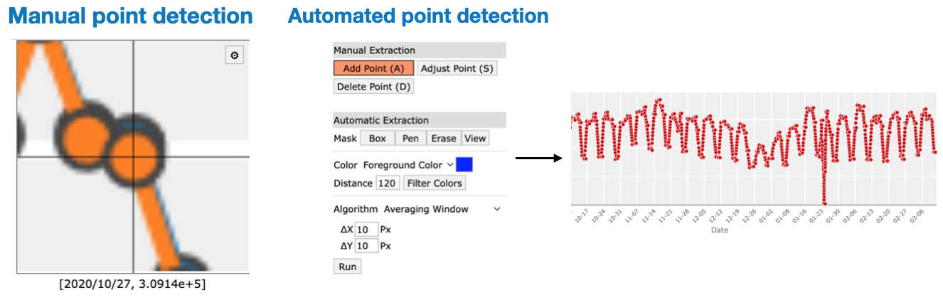
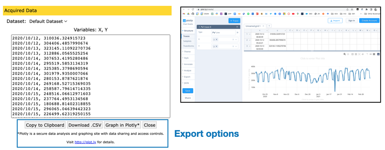
plot digitizers are a useful tool for extracting the raw numeric data from plots quickly