The concepts discussed today can be applied to any time-series, assuming there is “dense” enough sampling in the time dimension to resolve the oscillations.
We focus on sound as an example, since spectral analysis is often used for audio data.
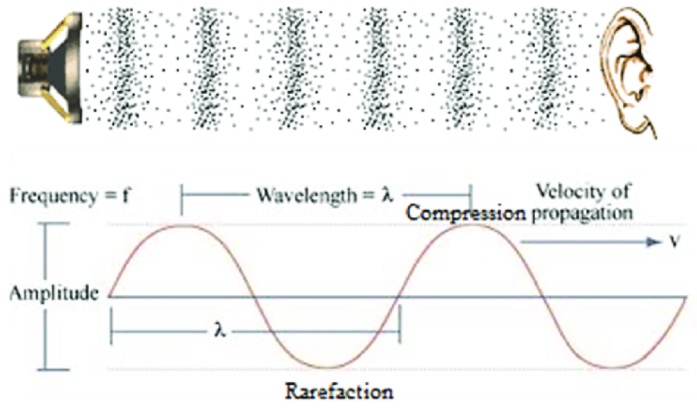
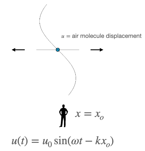
The simplest sound wave is a 1D planar sound wave: \(\,u(t)=u_{0}\sin(\omega t-kx_o)\)
It is helpful to imagine either time or position as constant to gain intuition about the wave
Analog vs digital
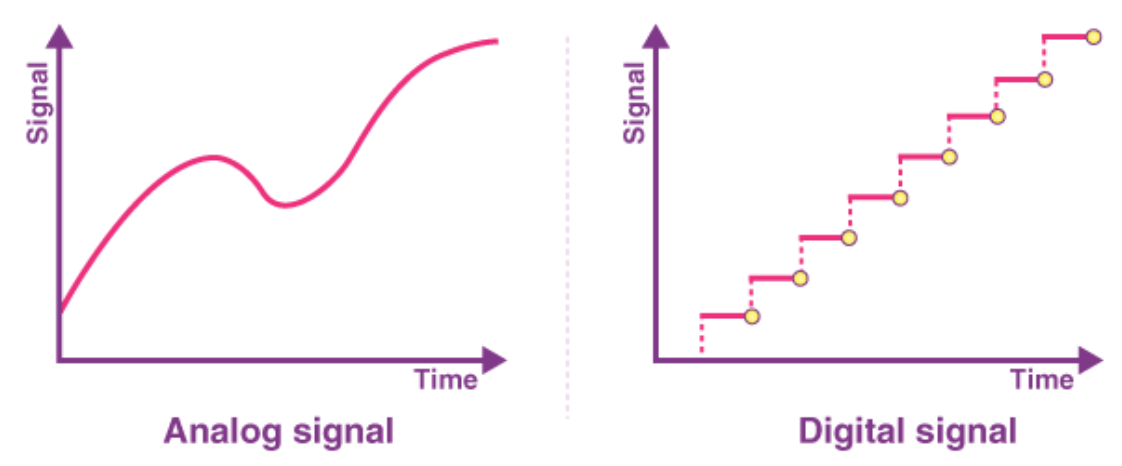
Analog signals are continuous and vary in amplitude and frequency while digital signals are discrete and represented as binary numbers \(\,\,\,\,\)
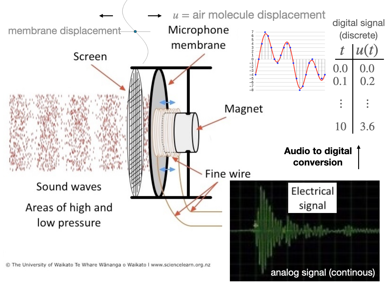
Data collection sensors, e.g. in your car, are generally analogue and measure continuous signals
This is because they measure continuous variations in some physical property, e.g. fluctuations in the EM field
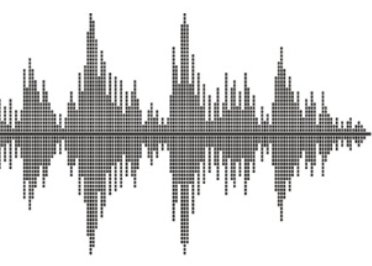
Audio signals
Let’s briefly consider how we capture and store sound data
Digital data and sampling rate
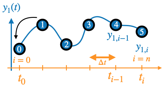
Due to RAM constraints, we sample a finite number of points when converting to digital
The frequency \(\frac{1}{\Delta t}\) of the sampling is defined by the sampling rate
Common options: 44.1kHz or 48kHz (48000 points per second)
Recording at 48kHz captures everything within the range of human hearing
Also facilitates compression: lower sampling rate has less data but lower quality
This means it takes up less spaces and easier to transfer over the internet
Vinyl Records are Analog, they contain the entire signal, resulting in high quality audio
Code: Creating a audio signal in python
Digital audio signals are commonly stored as numpy arrays
We can (1) read the audio into array from file (2) create waveform
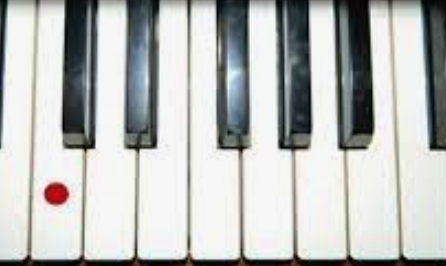
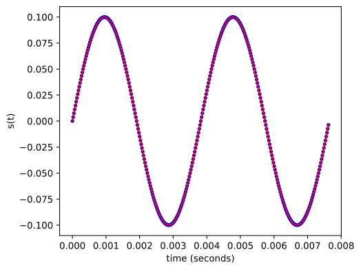
Here we create a signal for “middle C” on a piano “261.625565 hertz”
import numpy as npimport matplotlib.pyplot as pltf_C=261.626#SAMPLE RATER=44100#44.1kHz=standard sampling rate for audio #FUNCTION TO BUILD TIME-MESH BASED ON FREQUENCIESdef construct_mesh(f,N=2):#f=wave signal frequency, N=number of oscillationsglobal T,t,dt num_cycle=N# num_cycle=int(2.*f) T = num_cycle/f #total length of sound in seconds t = np.linspace(0,T,int(R*T)) t = t[0:-1] dt= t[1]-t[0];#TIMESTEP (seconds)#MIDDLE C: 261.625565 hertzconstruct_mesh(f_C)s =0.1*np.sin(2*np.pi*f_C*t)#SHOW INITIAL PART OF WAVEFORMfig, ax = plt.subplots(figsize=(5.5, 4.5))# plt.set_size_inches(18.5, 10.5)ax.plot(t[0:], s[0:], 'b.') ax.plot(t[0:], s[0:], 'r-') # ax.plot(t[0:NMAX], s[0:NMAX], 'b-') #AXIS LABELSax.set_xlabel('time (seconds)')ax.set_ylabel('s(t)')plt.show()
Nyquist frequency
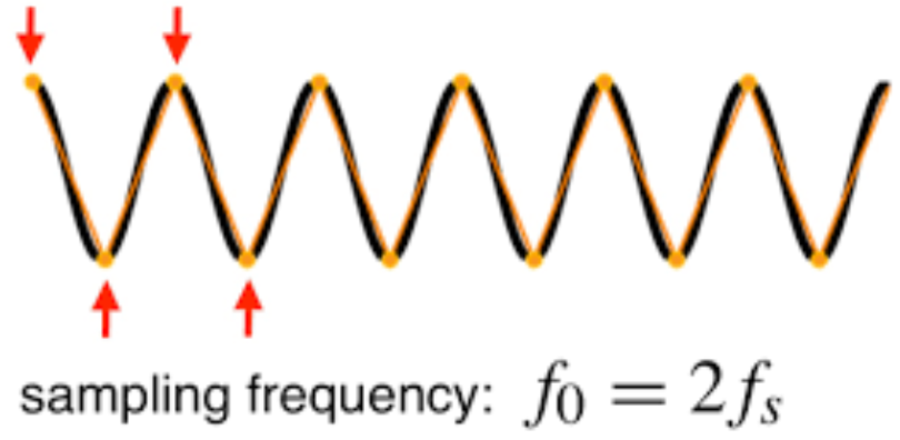
The Nyquist frequency is the highest frequency that can be accurately sampled in a digital signal processing system, and is half of the sampling rate.
Important: In spectral analysis you can’t sample sinusoidal contributions with frequencies lower than the Nyquist frequency
i.e. they maybe present in the “real world” signal, but will be truncated (invisible)
The loss of frequencies degrades the audio signal.
This is why digital audio sometimes sounds bad (over compressed)
Analog signal: example
Recording process:
String wave \(\rightarrow\) sound wave \(\rightarrow\) microphone membrane wave \(\rightarrow\) electrical wave \(\rightarrow\) waveform carved on Vinyl record
Listenting process:
waveform carved on Vinyl record \(\rightarrow\) electrical wave \(\rightarrow\) speaker membrane wave \(\rightarrow\) sound wave \(\rightarrow\) human ear
Fun aside: Video sampling
Note: Sampling rate is also fundamental to capturing video image data
Super-position
superposition: For certain systems, the net response caused by two or more stimuli is the sum of the responses that would have been caused by each stimulus individually
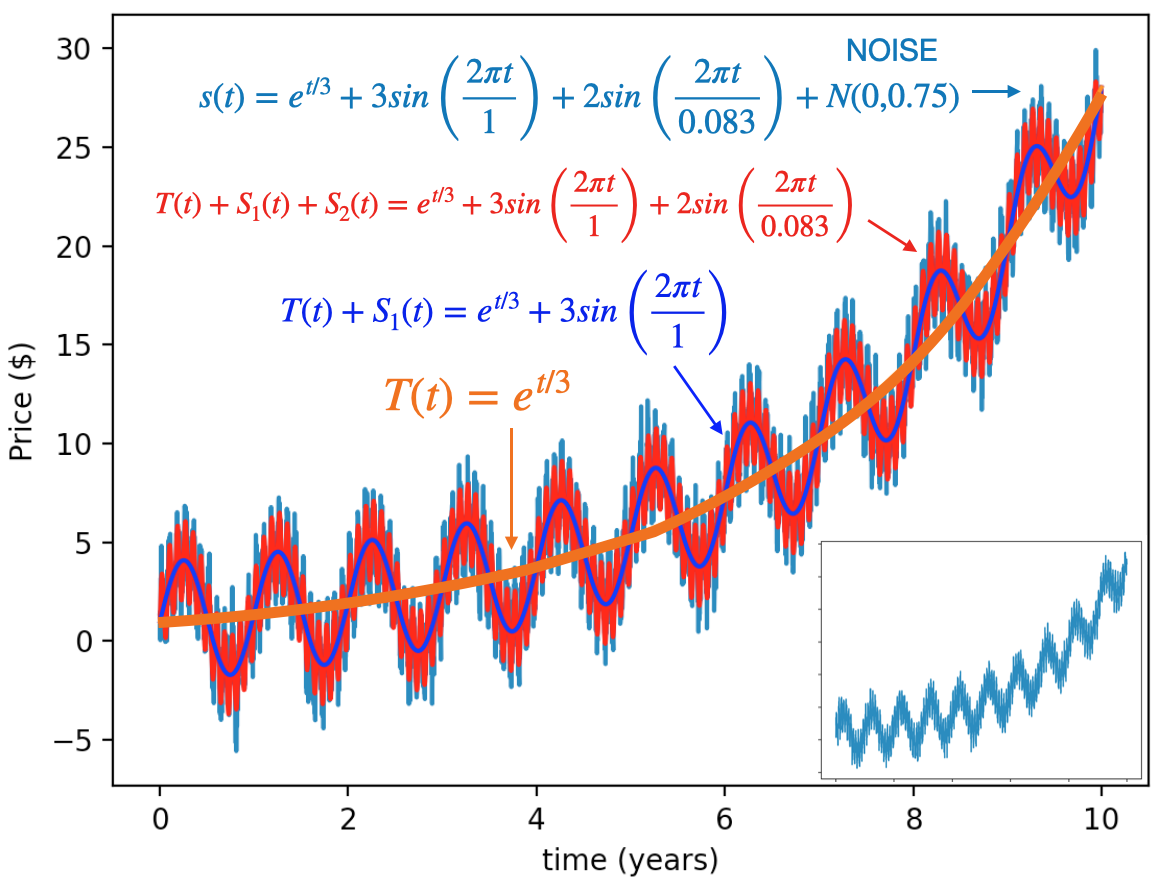
Often time-series can be decomposed as an additive superposition of components.
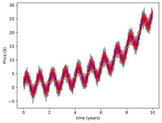
import matplotlib.pyplot as pltimport numpy as np# TIME POINTS: UNITS YEARS # (10 years sampled daily)t = np.linspace(0.0, 10.0, 365*10)N =len(t)# TIMESERIES COMPONENTS#non-linear trendtrend=np.exp(t/3) #seaonality: period of 1 year, amplitude of 3season_1=3*np.sin(2*np.pi*t/(1)) #seaonality: period of 1/12 years (monthly), A=2season_2=2*np.sin(2*np.pi*t/(1/12.)) noise=np.random.normal(0,0.75,N)# COMBINE COMPONENTStimeseries = trend+season_1+season_2+noise# PLOT fig, ax = plt.subplots()ax.plot(t, timeseries)ax.plot(t, trend+season_1+season_2,'-r')ax.plot(t, trend+season_1,'-b')ax.plot(t, trend)ax.set(xlabel='time (years)', ylabel='Price ($)')plt.show()
Audio superposition
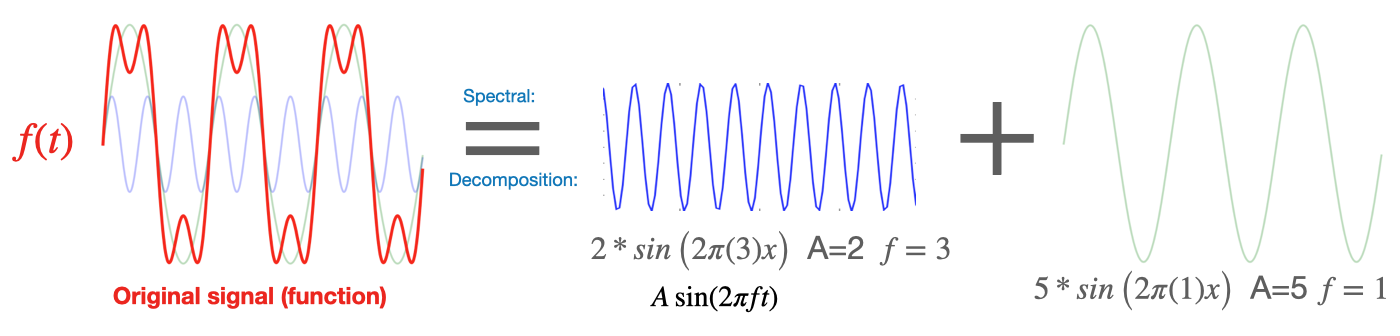
Superposition occurs in audio signals, the total sound wave is the sum (superposition) of many sine and cosine terms with differing frequencies and amplitudes
As we will see later in the lecture, this concept of superposition is completely fundamental to spectral analysis.
It also occurs in many physical phenomena, for example, water waves
Code demo: Exploring sound data
See sound-example/sound.ipynb if you want to follow along.
Fourier series and transforms
Introduction
Fourier Series: general idea
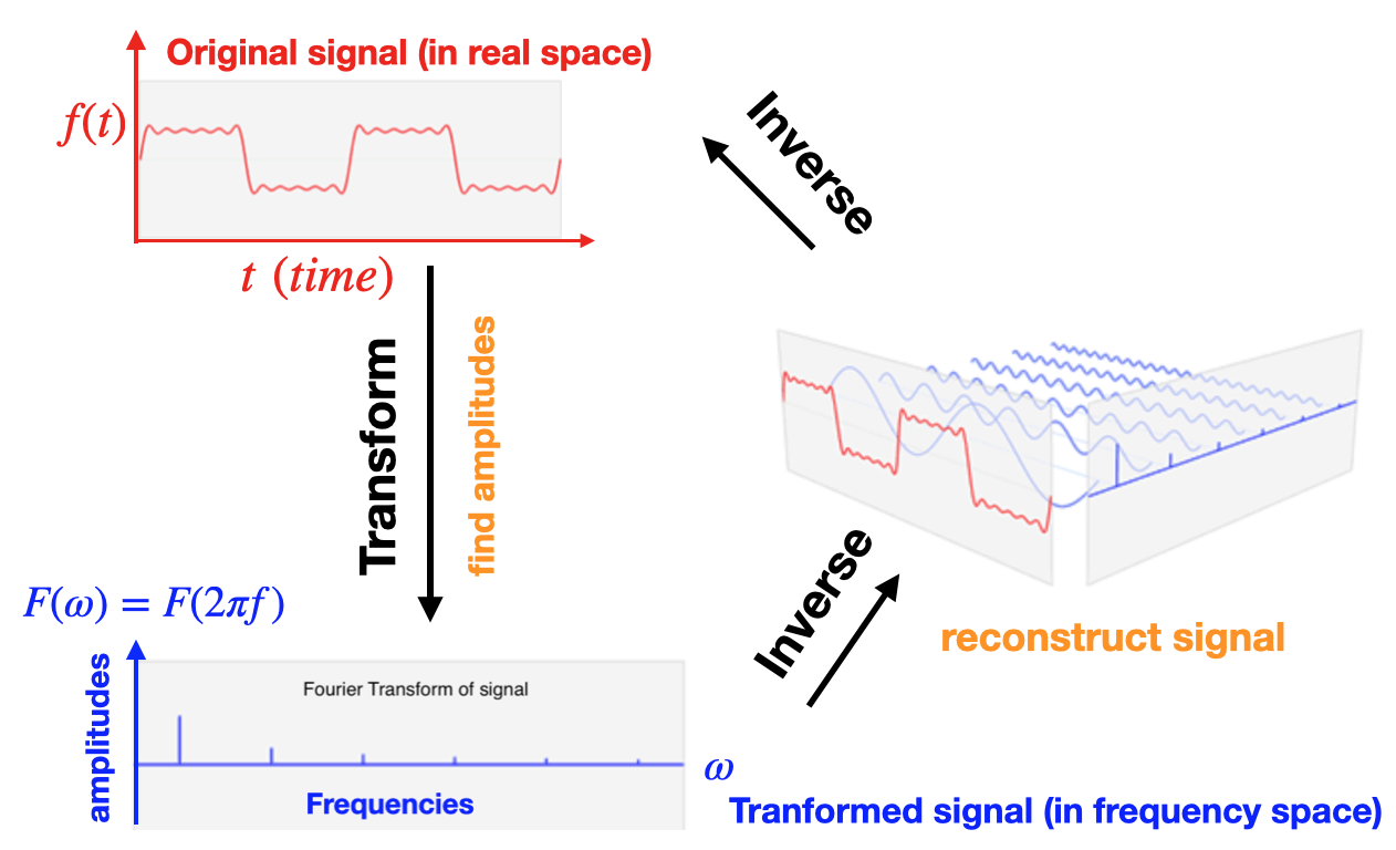
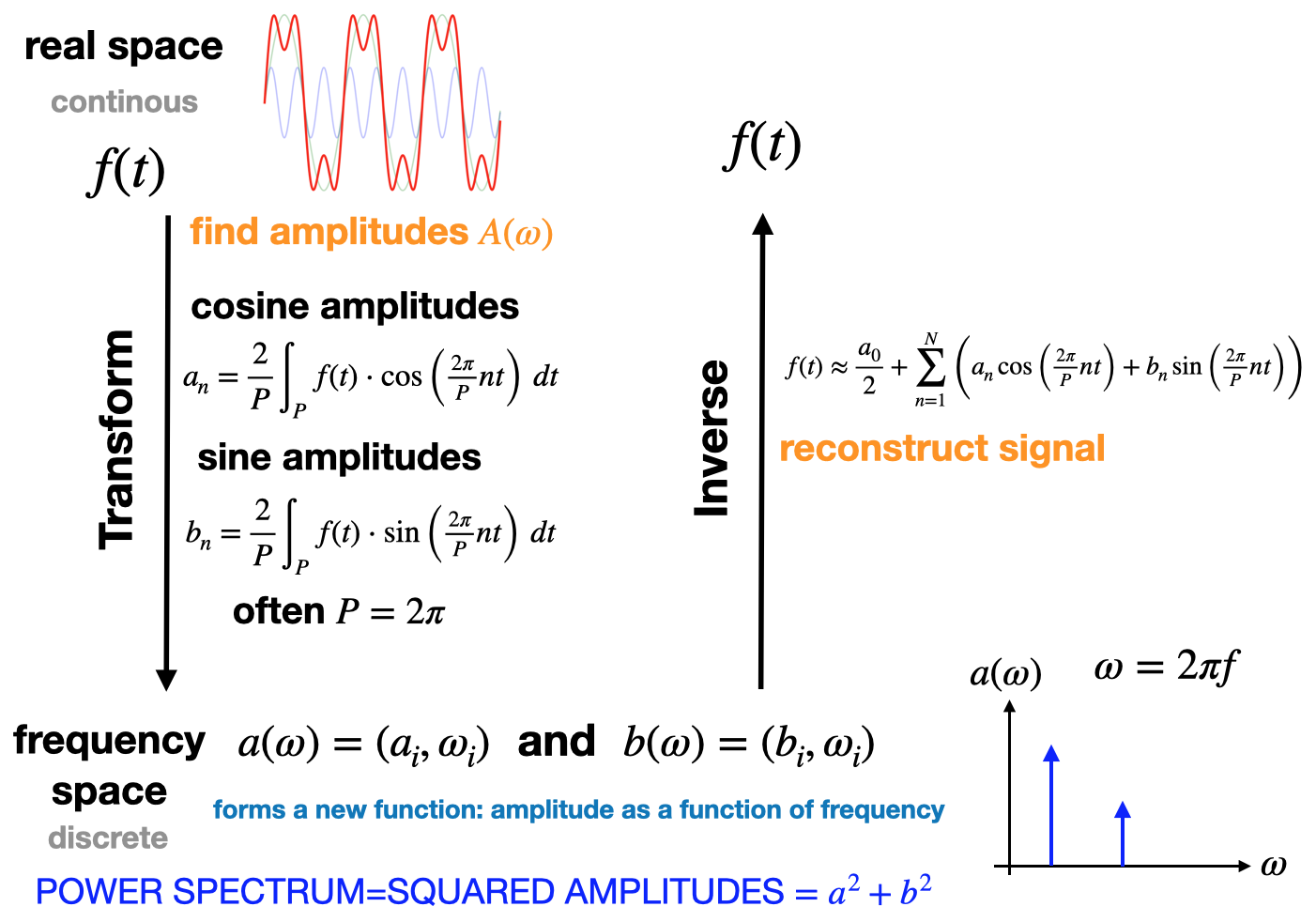
The Fourier Series decomposes functions into a sum of sine and cosine terms with differing frequencies and amplitudes
The original function \(f(t)\), is called the “real space representation” and is continuous
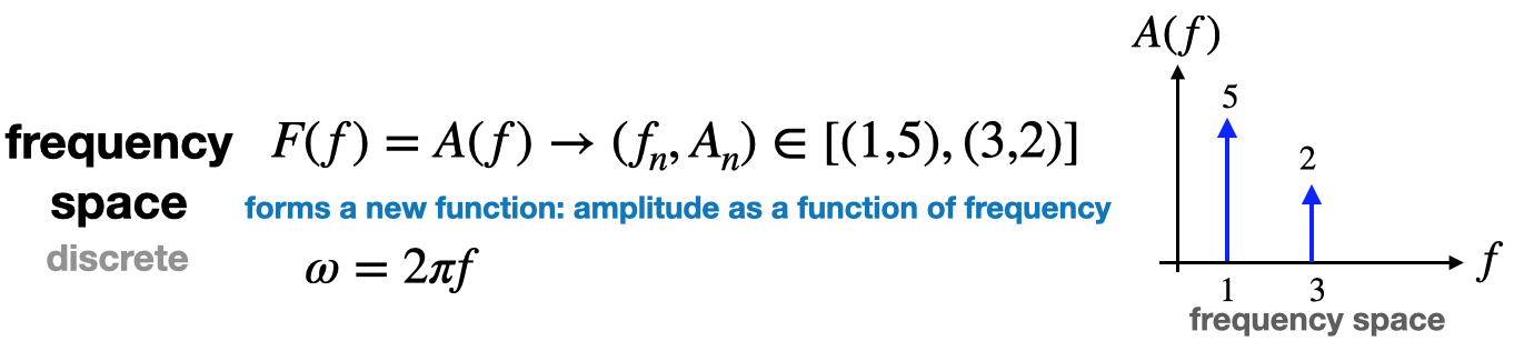
The transformed function \(F(\omega)\), is called the “frequency representation” and is discrete
The inverse transform re-construct \(f(t)\) from \(F(\omega)\) given amplitudes&frequencies
Fourier transform: general idea
Fourier transform decompose functions into a sum (superposition) of sine and cosine terms with differing frequencies and amplitudes
Math: Fourier series Real form
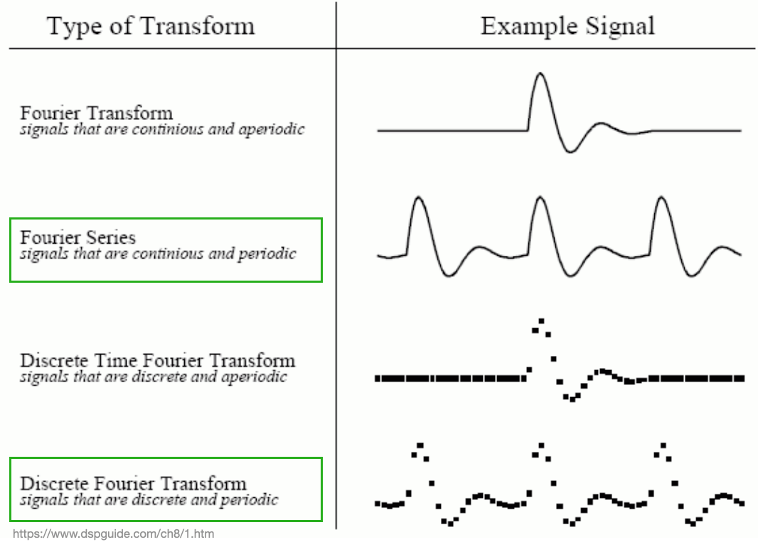
Four types of Fourier transforms:
Math: Four types of Fourier transforms:
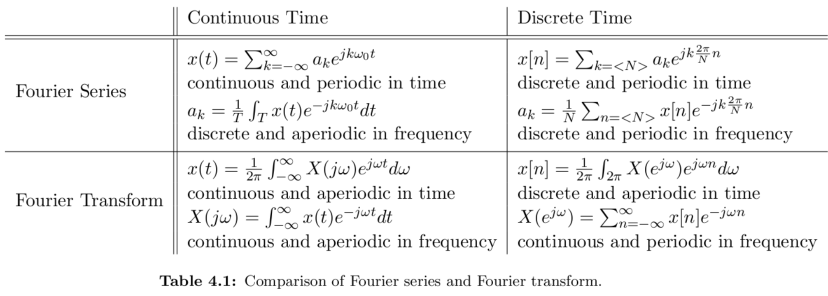
Here are the mathematical formulae for the four different transforms
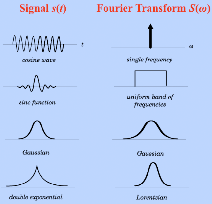
Example
Notice that localized objects in real space become “spread-out” in frequency space
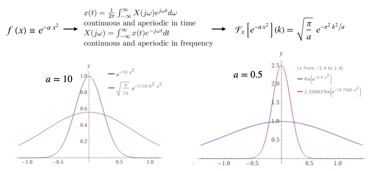
Example: Fourier Transform of Gaussian (FIX)
signals that are Continuous and aperiodic use the “Fourier transform”
Again, note that localized objects in real space become “spread-out” in frequency space
Code demo: Exploring sound data
See spectral-example/spectral.ipynb if you want to follow along.