%matplotlib inline
from IPython.display import Image
Image('images/figure-1.png', width = 600, height = 600)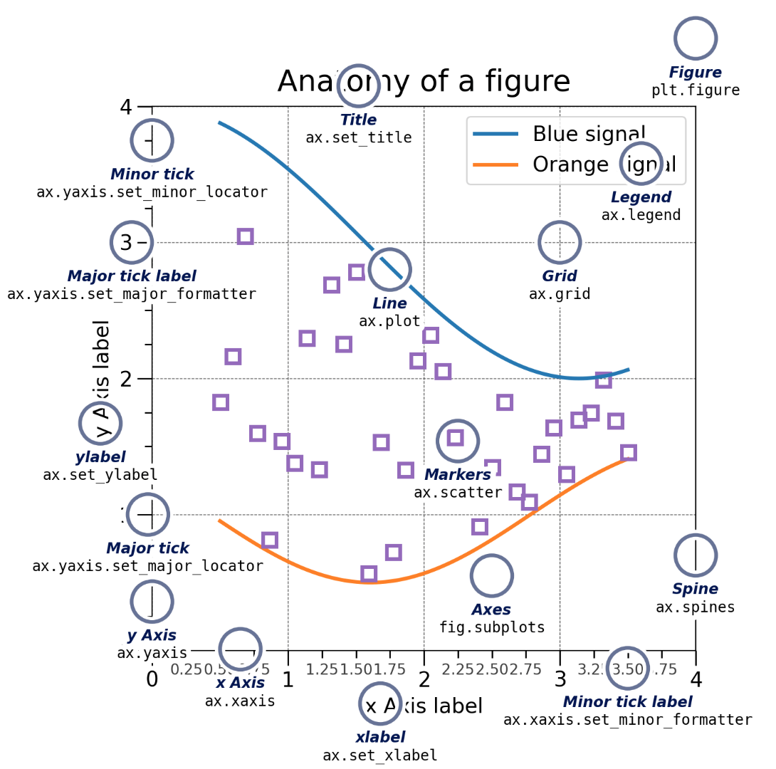
When making professional level plots, it is very important to adhere to the following guidelines (at a minimum):
Failure to adhere to these guidelines will consistently lose you points in any class you take in the DSAN program.
Matplotlib can be installed using either pip or conda by running the following commands from the command line.
python -m pip install matplotlib
conda install matplotlib
All plotting functions expect np.array or np.ma.masked_array as input.
Classes that are ‘array-like’ such as pandas data objects and np.matrix may or may not work as intended.
It is best to convert these to np.array objects prior to plotting.
Run the following cell to see the various key components of a MPL figure
%matplotlib inline
from IPython.display import Image
Image('images/figure-1.png', width = 600, height = 600)
In matplotlib there are two important object types, the figure object and the axes object.
This sometimes leads to confusion, because you will see code that uses axes objects commands and sometimes not.
So what is the difference between these two objects?
Figures (canvas)
Axes (individual plots)
The following figure exemplifies the difference between the two types of objects.
%matplotlib inline
from IPython.display import Image
Image('images/figure-2.png', width = 1000, height = 500)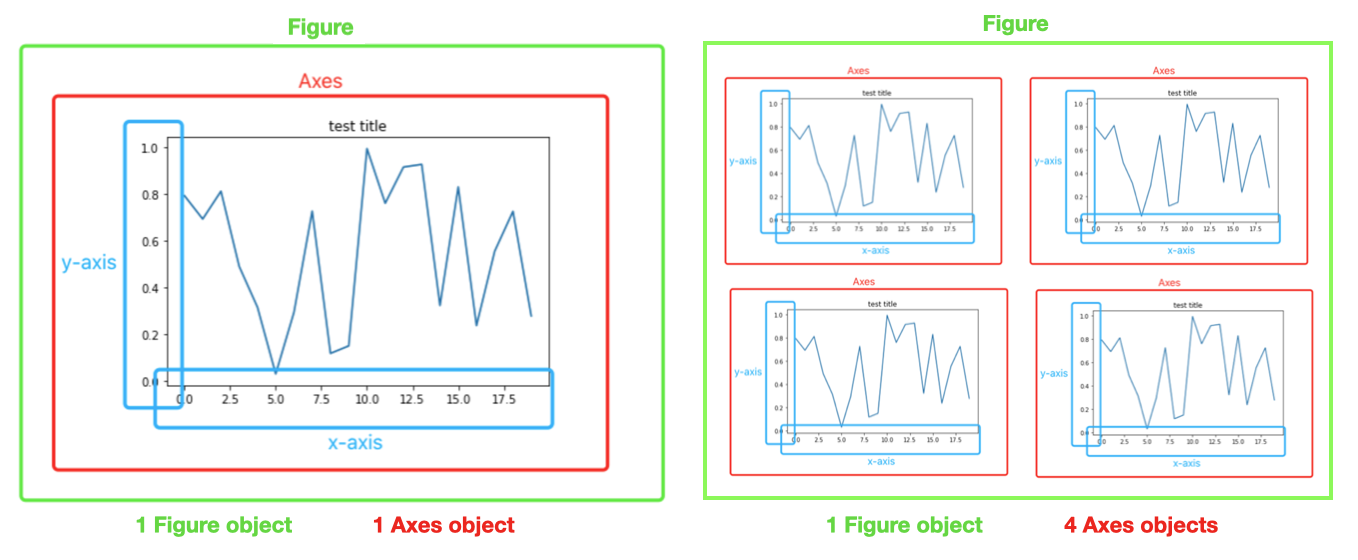
Because of these two object types, there are essentially two ways to use Matplotlib: * Method-1) Rely on pyplot to automatically create and manage the Figures and Axes, and use pyplot functions for plotting. * Method-2) Explicitly create Figures and Axes, and call methods on them (i.e. the “object-oriented (OO) style”).
import matplotlib.pyplot as plt
import numpy as np

#DEFINE DATA
x=[1, 2, 3, 4]
y=[1, 2, 3, 4]

#PLOT
plt.plot(x,y,'o') # 'o' makes a scatterplot or point plot
plt.show()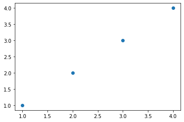
IMPORTANT NOTE: * When using a Jupiter notebook (.ipynb), you do not need to explicitly tell the code to render the plot by using the “plt.show()” command. * However, when using standard python (.py), you do need to include the command, otherwise the plot will not render. * Therefore, we include the command below for completeness sake * The same is true regarding printing to the screen. * A standard python code (.py) will not print, unless the print() command is explicitly called.
For completeness sake, we will frequently repeat the import commands, so that the code chunks are self-contained.
Basic customization
import matplotlib.pyplot as plt

#DEFINE DATA
x=[1, 2, 3, 4]
y=[1, 2, 3, 4]

#PLOT
plt.plot(x,y,'-o') # '-o' makes plots points and a line

#SET FIGURE LABELS AND TITLE
FS=20
plt.suptitle("Newton's Law: F=ma", fontsize=FS)
plt.xlabel('Acceleration (m/s/s)', fontsize=FS)
plt.ylabel('Force (N)', fontsize=FS)
#TUPLE SPECIFIES WHERE TO PUT ANNOTATION
plt.annotate("slope=mass (kg)", (1,3.65), fontsize=FS)
plt.show()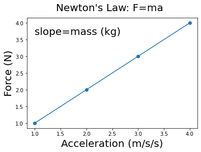
import matplotlib.pyplot as plt
import numpy as np

#DEFINE DATA
x=[1, 2, 3, 4]
y=[1, 2, 3, 4]

#DEFINE OBJECTS
fig, ax = plt.subplots()

#PLOT
ax.plot(x,y,'o')
plt.show()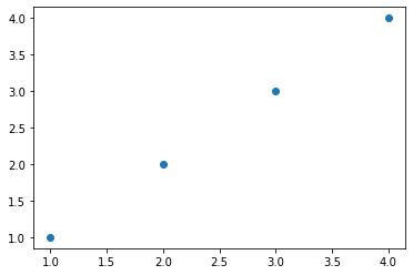
Basic customization * Just as with method-1, we can do various forms of customization. * However notice that some of the commands are different, since we are acting on the axis object.
import matplotlib.pyplot as plt
import numpy as np

#DEFINE DATA
x=[1, 2, 3, 4]
y=[1, 2, 3, 4]

#DEFINE OBJECTS
fig, ax = plt.subplots()

#PLOT
ax.plot(x,y,'-o')

#CUSTOMIZE
FS=20
ax.set_title("Newton's Law: F=ma", fontsize=FS)
ax.set_xlabel('Acceleration (m/s/s)', fontsize=FS)
ax.set_ylabel('Force (N)', fontsize=FS)
ax.annotate("slope=mass (kg)", (1,3.65), fontsize=FS)
plt.show()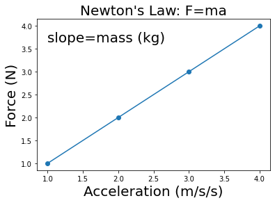
Typically, the default properties of plots are unacceptable for professional-level presentations.
This is because the labels are not very intuitive, lack units, and have fonts that are too small.
Therefore, we often want to modify them to generate higher-quality visualizations.
The default parameters of MPL are stored in an object called rcParams which is similar to a dictionary
Therefore, there are essentially four ways to customize Matplotlib:
NOTE: Setting rcParams at runtime takes precedence over style sheets, style sheets take precedence over matplotlibrc files.
You can print the defaults in the rcParams object, as shown below.
print(plt.rcParams)_internal.classic_mode: False
agg.path.chunksize: 0
animation.bitrate: -1
animation.codec: h264
animation.convert_args: []
animation.convert_path: convert
animation.embed_limit: 20.0
animation.ffmpeg_args: []
animation.ffmpeg_path: ffmpeg
animation.frame_format: png
animation.html: none
animation.writer: ffmpeg
axes.autolimit_mode: data
axes.axisbelow: line
axes.edgecolor: black
axes.facecolor: white
axes.formatter.limits: [-5, 6]
axes.formatter.min_exponent: 0
axes.formatter.offset_threshold: 4
axes.formatter.use_locale: False
axes.formatter.use_mathtext: False
axes.formatter.useoffset: True
axes.grid: False
axes.grid.axis: both
axes.grid.which: major
axes.labelcolor: black
axes.labelpad: 4.0
axes.labelsize: medium
axes.labelweight: normal
axes.linewidth: 0.8
axes.prop_cycle: cycler('color', ['#1f77b4', '#ff7f0e', '#2ca02c', '#d62728', '#9467bd', '#8c564b', '#e377c2', '#7f7f7f', '#bcbd22', '#17becf'])
axes.spines.bottom: True
axes.spines.left: True
axes.spines.right: True
axes.spines.top: True
axes.titlecolor: auto
axes.titlelocation: center
axes.titlepad: 6.0
axes.titlesize: large
axes.titleweight: normal
axes.titley: None
axes.unicode_minus: True
axes.xmargin: 0.05
axes.ymargin: 0.05
axes.zmargin: 0.05
axes3d.grid: True
backend: module://matplotlib_inline.backend_inline
backend_fallback: True
boxplot.bootstrap: None
boxplot.boxprops.color: black
boxplot.boxprops.linestyle: -
boxplot.boxprops.linewidth: 1.0
boxplot.capprops.color: black
boxplot.capprops.linestyle: -
boxplot.capprops.linewidth: 1.0
boxplot.flierprops.color: black
boxplot.flierprops.linestyle: none
boxplot.flierprops.linewidth: 1.0
boxplot.flierprops.marker: o
boxplot.flierprops.markeredgecolor: black
boxplot.flierprops.markeredgewidth: 1.0
boxplot.flierprops.markerfacecolor: none
boxplot.flierprops.markersize: 6.0
boxplot.meanline: False
boxplot.meanprops.color: C2
boxplot.meanprops.linestyle: --
boxplot.meanprops.linewidth: 1.0
boxplot.meanprops.marker: ^
boxplot.meanprops.markeredgecolor: C2
boxplot.meanprops.markerfacecolor: C2
boxplot.meanprops.markersize: 6.0
boxplot.medianprops.color: C1
boxplot.medianprops.linestyle: -
boxplot.medianprops.linewidth: 1.0
boxplot.notch: False
boxplot.patchartist: False
boxplot.showbox: True
boxplot.showcaps: True
boxplot.showfliers: True
boxplot.showmeans: False
boxplot.vertical: True
boxplot.whiskerprops.color: black
boxplot.whiskerprops.linestyle: -
boxplot.whiskerprops.linewidth: 1.0
boxplot.whiskers: 1.5
contour.corner_mask: True
contour.linewidth: None
contour.negative_linestyle: dashed
date.autoformatter.day: %Y-%m-%d
date.autoformatter.hour: %m-%d %H
date.autoformatter.microsecond: %M:%S.%f
date.autoformatter.minute: %d %H:%M
date.autoformatter.month: %Y-%m
date.autoformatter.second: %H:%M:%S
date.autoformatter.year: %Y
date.converter: auto
date.epoch: 1970-01-01T00:00:00
date.interval_multiples: True
docstring.hardcopy: False
errorbar.capsize: 0.0
figure.autolayout: False
figure.constrained_layout.h_pad: 0.04167
figure.constrained_layout.hspace: 0.02
figure.constrained_layout.use: False
figure.constrained_layout.w_pad: 0.04167
figure.constrained_layout.wspace: 0.02
figure.dpi: 72.0
figure.edgecolor: (1, 1, 1, 0)
figure.facecolor: (1, 1, 1, 0)
figure.figsize: [6.0, 4.0]
figure.frameon: True
figure.max_open_warning: 20
figure.raise_window: True
figure.subplot.bottom: 0.125
figure.subplot.hspace: 0.2
figure.subplot.left: 0.125
figure.subplot.right: 0.9
figure.subplot.top: 0.88
figure.subplot.wspace: 0.2
figure.titlesize: large
figure.titleweight: normal
font.cursive: ['Apple Chancery', 'Textile', 'Zapf Chancery', 'Sand', 'Script MT', 'Felipa', 'Comic Neue', 'Comic Sans MS', 'cursive']
font.family: ['sans-serif']
font.fantasy: ['Chicago', 'Charcoal', 'Impact', 'Western', 'Humor Sans', 'xkcd', 'fantasy']
font.monospace: ['DejaVu Sans Mono', 'Bitstream Vera Sans Mono', 'Computer Modern Typewriter', 'Andale Mono', 'Nimbus Mono L', 'Courier New', 'Courier', 'Fixed', 'Terminal', 'monospace']
font.sans-serif: ['DejaVu Sans', 'Bitstream Vera Sans', 'Computer Modern Sans Serif', 'Lucida Grande', 'Verdana', 'Geneva', 'Lucid', 'Arial', 'Helvetica', 'Avant Garde', 'sans-serif']
font.serif: ['DejaVu Serif', 'Bitstream Vera Serif', 'Computer Modern Roman', 'New Century Schoolbook', 'Century Schoolbook L', 'Utopia', 'ITC Bookman', 'Bookman', 'Nimbus Roman No9 L', 'Times New Roman', 'Times', 'Palatino', 'Charter', 'serif']
font.size: 10.0
font.stretch: normal
font.style: normal
font.variant: normal
font.weight: normal
grid.alpha: 1.0
grid.color: #b0b0b0
grid.linestyle: -
grid.linewidth: 0.8
hatch.color: black
hatch.linewidth: 1.0
hist.bins: 10
image.aspect: equal
image.cmap: viridis
image.composite_image: True
image.interpolation: antialiased
image.lut: 256
image.origin: upper
image.resample: True
interactive: True
keymap.back: ['left', 'c', 'backspace', 'MouseButton.BACK']
keymap.copy: ['ctrl+c', 'cmd+c']
keymap.forward: ['right', 'v', 'MouseButton.FORWARD']
keymap.fullscreen: ['f', 'ctrl+f']
keymap.grid: ['g']
keymap.grid_minor: ['G']
keymap.help: ['f1']
keymap.home: ['h', 'r', 'home']
keymap.pan: ['p']
keymap.quit: ['ctrl+w', 'cmd+w', 'q']
keymap.quit_all: []
keymap.save: ['s', 'ctrl+s']
keymap.xscale: ['k', 'L']
keymap.yscale: ['l']
keymap.zoom: ['o']
legend.borderaxespad: 0.5
legend.borderpad: 0.4
legend.columnspacing: 2.0
legend.edgecolor: 0.8
legend.facecolor: inherit
legend.fancybox: True
legend.fontsize: medium
legend.framealpha: 0.8
legend.frameon: True
legend.handleheight: 0.7
legend.handlelength: 2.0
legend.handletextpad: 0.8
legend.labelcolor: None
legend.labelspacing: 0.5
legend.loc: best
legend.markerscale: 1.0
legend.numpoints: 1
legend.scatterpoints: 1
legend.shadow: False
legend.title_fontsize: None
lines.antialiased: True
lines.color: C0
lines.dash_capstyle: butt
lines.dash_joinstyle: round
lines.dashdot_pattern: [6.4, 1.6, 1.0, 1.6]
lines.dashed_pattern: [3.7, 1.6]
lines.dotted_pattern: [1.0, 1.65]
lines.linestyle: -
lines.linewidth: 1.5
lines.marker: None
lines.markeredgecolor: auto
lines.markeredgewidth: 1.0
lines.markerfacecolor: auto
lines.markersize: 6.0
lines.scale_dashes: True
lines.solid_capstyle: projecting
lines.solid_joinstyle: round
markers.fillstyle: full
mathtext.bf: sans:bold
mathtext.cal: cursive
mathtext.default: it
mathtext.fallback: cm
mathtext.fontset: dejavusans
mathtext.it: sans:italic
mathtext.rm: sans
mathtext.sf: sans
mathtext.tt: monospace
patch.antialiased: True
patch.edgecolor: black
patch.facecolor: C0
patch.force_edgecolor: False
patch.linewidth: 1.0
path.effects: []
path.simplify: True
path.simplify_threshold: 0.111111111111
path.sketch: None
path.snap: True
pcolor.shading: auto
pcolormesh.snap: True
pdf.compression: 6
pdf.fonttype: 3
pdf.inheritcolor: False
pdf.use14corefonts: False
pgf.preamble:
pgf.rcfonts: True
pgf.texsystem: xelatex
polaraxes.grid: True
ps.distiller.res: 6000
ps.fonttype: 3
ps.papersize: letter
ps.useafm: False
ps.usedistiller: None
savefig.bbox: None
savefig.directory: ~
savefig.dpi: figure
savefig.edgecolor: auto
savefig.facecolor: auto
savefig.format: png
savefig.orientation: portrait
savefig.pad_inches: 0.1
savefig.transparent: False
scatter.edgecolors: face
scatter.marker: o
svg.fonttype: path
svg.hashsalt: None
svg.image_inline: True
text.antialiased: True
text.color: black
text.hinting: force_autohint
text.hinting_factor: 8
text.kerning_factor: 0
text.latex.preamble:
text.usetex: False
timezone: UTC
tk.window_focus: False
toolbar: toolbar2
webagg.address: 127.0.0.1
webagg.open_in_browser: True
webagg.port: 8988
webagg.port_retries: 50
xaxis.labellocation: center
xtick.alignment: center
xtick.bottom: True
xtick.color: black
xtick.direction: out
xtick.labelbottom: True
xtick.labelcolor: inherit
xtick.labelsize: medium
xtick.labeltop: False
xtick.major.bottom: True
xtick.major.pad: 3.5
xtick.major.size: 3.5
xtick.major.top: True
xtick.major.width: 0.8
xtick.minor.bottom: True
xtick.minor.pad: 3.4
xtick.minor.size: 2.0
xtick.minor.top: True
xtick.minor.visible: False
xtick.minor.width: 0.6
xtick.top: False
yaxis.labellocation: center
ytick.alignment: center_baseline
ytick.color: black
ytick.direction: out
ytick.labelcolor: inherit
ytick.labelleft: True
ytick.labelright: False
ytick.labelsize: medium
ytick.left: True
ytick.major.left: True
ytick.major.pad: 3.5
ytick.major.right: True
ytick.major.size: 3.5
ytick.major.width: 0.8
ytick.minor.left: True
ytick.minor.pad: 3.4
ytick.minor.right: True
ytick.minor.size: 2.0
ytick.minor.visible: False
ytick.minor.width: 0.6
ytick.right: False# OR YOU CAN PRINT INDIVIDUAL DEFAULT ATTRIBUTES
print(plt.rcParams["figure.figsize"])[6.0, 4.0]# YOU CAN ALSO MODIFY THESE ATTRIBUTES
plt.rcParams["figure.figsize"]= (10,10) # change the default figure size to a 10in x 10in resolution
print(plt.rcParams["figure.figsize"])[10.0, 10.0]This modification will effect all future plots, unless we change it back.
Or until we restart the python kernel, e.g. by reopening the .ipynb file or re-running the .py file, which will restore the un-modified defaults.
#RESET TO ORIGINAL DEFAULTS
plt.rcParams["figure.figsize"]= (6,4)
print(plt.rcParams["figure.figsize"])
[6.0, 4.0]The following example shows various ways to manually modify attributes of your plot when you create it (i.e. method-4).
These modifications do not change the MPL defaults in rcParams.
These customization options can be used to make a professional looking graph.
IMPORTANT NOTE: At the bottom of the code, there are various commands that can print the plot to a file using different file formats.
import matplotlib.pyplot as plt
import numpy as np

#GENERATE DATA
N=500   #number of data points
x=np.linspace(-45,45.0, N);
ye=x*x*np.sin(x) #exact
y=ye+np.random.normal(0, 200, N) #add noise

#FONT SIZE
FS=22

#DEFINE FIG+AX OBJECTS
fig, ax = plt.subplots()
#https://www.canva.com/colors/color-wheel/
ax.plot(x,y,'o',color='#FF0012', markersize=16, label='Data')
ax.plot(x,ye, color='#0012FF'  ,linewidth=6, label='Ground truth')
ax.plot(x,ye,color='#12FF00'   , linewidth=1, linestyle='dashed')

#SET LEGEND
ax.legend(fontsize=FS)

#SET FIGURE SIZE
fig.set_size_inches(10, 10)

#FIGURE TITLE
fig.suptitle('Decaying harmonic oscillations', fontsize=24)

#AXIS LABELS
ax.set_xlabel('Time (ps)', fontsize=FS)
ax.set_ylabel('Amplitude (cm)', fontsize=FS)

# #X-Y PLOT RANGE
ax.set_xlim([-40,0])
ax.set_ylim([-1750,1750])

#AXIS TIC VALUES
ax.set_xticks([-40,-30,-20,-10,0],fontsize=20)
ax.set_yticks([-2000,-1000,0,1000,2000],fontsize=20)

#CONTROL AXIS TICK FORMAT
ax.yaxis.set_major_formatter(plt.FormatStrFormatter('%4.2f'))
ax.xaxis.set_major_formatter(plt.FormatStrFormatter('%.1f'))

#AXIS TIC FONT SIZE
ax.tick_params(axis='both', which='major', labelsize=FS)
ax.tick_params(axis='both', which='minor', labelsize=FS)

# #SAVE IMAGES TO A FILE
fig.savefig('plot-1.png', bbox_inches='tight')
# f.savefig("plot-1.pdf", bbox_inches='tight')
# f.savefig("plot-1.eps", bbox_inches='tight')

#RENDER AND SHOW IMAGE
plt.show()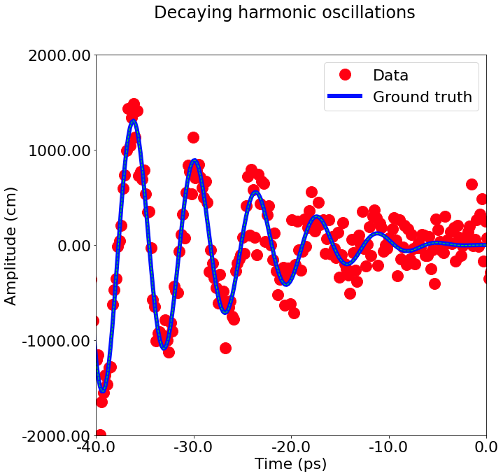
fig, ax = plt.subplots(figsize=(5, 2.7))
ax.scatter(x, y, s=50, facecolor='#FF0000', edgecolor='#000000');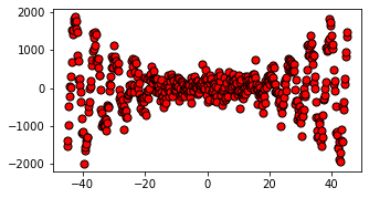
There are also various color palettes included with MPL. More information about color palettes be found at the following link * https://matplotlib.org/3.5.0/tutorials/colors/colormaps.html
Line widths are typically in typographic points \((1 pt = \frac{1}{72}inch)\) and available for Artists that have stroked lines. Similarly, stroked lines can have a linestyle. See the linestyles example.
Marker size depends on the method being used. plot specifies markersize in points, and is generally the “diameter” or width of the marker. scatter specifies markersize as approximately proportional to the visual area of the marker. There is an array of markerstyles available as string codes (see markers), or users can define their own MarkerStyle (see Marker reference):
fig, ax = plt.subplots(figsize=(5, 2.7))
ax.plot(x, 'o', label='x1')
ax.plot(x+250, 'd', label='x2')
ax.plot(x+500, 'v', label='x3')
ax.plot(x+1000, 's', label='x4')
ax.legend();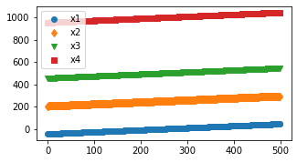
set_xlabel, set_ylabel, and set_title are used to add text in the indicated locations (see Text in Matplotlib Plots for more discussion). Text can also be directly added to plots using text:
All of the text functions return a matplotlib.text.Text instance. Just as with lines above, you can customize the properties by passing keyword arguments into the text functions:
mu, sigma = 115, 15
x = mu + sigma * np.random.randn(10000)
fig, ax = plt.subplots(figsize=(5, 2.7), layout='constrained')
# the histogram of the data
n, bins, patches = ax.hist(x, 50, density=1, facecolor='C0', alpha=0.75)

ax.set_xlabel('Length [cm]')
ax.set_ylabel('Probability')
ax.set_title('Aardvark lengths\n (not really)')
ax.text(75, .025, r'$\mu=115,\ \sigma=15$')
ax.axis([55, 175, 0, 0.03])      # sets x and y limits of the figure axes
ax.grid(True);                   # add gridlines to plot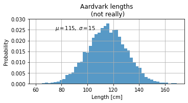
If we want to include multiple subplots in one figure (known as faceting), then we need to define multiple axes objects.
The individual axes objects can be modified using the standard indexing formalism discussed for lists in a previous lesson.
The following examples demonstrates the generation of subplots.
import matplotlib.pyplot as plt
import numpy as np

# Some example data to display
x = np.linspace(0, 2 * np.pi, 400)
y = np.sin(x ** 2)

#EXAMPLE-1
fig, ax = plt.subplots()
ax.plot(x, y)
ax.set_title('A single plot')
Text(0.5, 1.0, 'A single plot')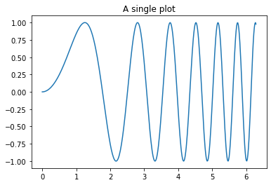
#EXAMPLE-2
fig, axs = plt.subplots(2)
fig.suptitle('Vertically stacked subplots')
axs[0].plot(x, y)
axs[1].plot(x, -y)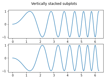
#EXAMPLE-3

fig, (ax1, ax2) = plt.subplots(1, 2)
fig.suptitle('Horizontally stacked subplots')
ax1.plot(x, y)
ax2.plot(x, -y)

#INCREASE FIGURE SIZE
fig.set_size_inches(15, 5)
plt.show()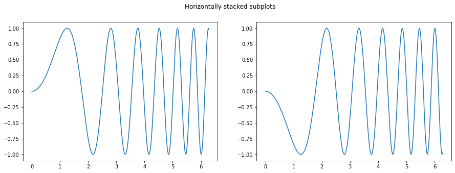
#EXAMPLE-4
fig, axs = plt.subplots(2, 2)
axs[0, 0].plot(x, y)
axs[0, 0].set_title('Axis [0, 0]')
axs[0, 1].plot(x, y, 'tab:orange')
axs[0, 1].set_title('Axis [0, 1]')
axs[1, 0].plot(x, -y, 'tab:green')
axs[1, 0].set_title('Axis [1, 0]')
axs[1, 1].plot(x, -y, 'tab:red')
axs[1, 1].set_title('Axis [1, 1]')

for ax in axs.flat:
    ax.set(xlabel='x-label', ylabel='y-label')

# Hide x labels and tick labels for top plots and y ticks for right plots.
for ax in axs.flat:
    ax.label_outer()

#INCREASE FIGURE SIZE
fig.set_size_inches(10, 10)
plt.show()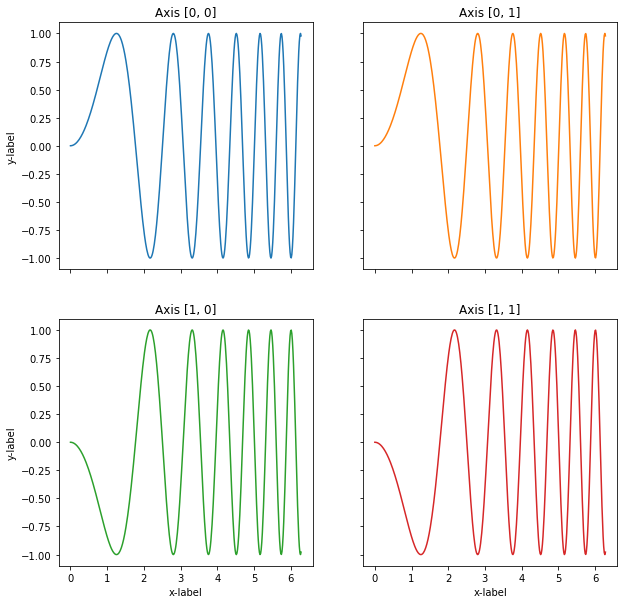
#EXAMPLE-5
import matplotlib.pyplot as plt
import numpy as np

n_rows = 2
n_cols = 2
#INITIALIZE
fig, axes = plt.subplots(n_rows, n_cols)

#INCREASE FIGURE SIZE
fig.set_size_inches(15, 10)

#POPULATE ROW AND COLUMN AXES OBJECT
for row_num in range(n_rows):
    for col_num in range(n_cols):
        #AXES (CELL) ATTRIBUTES
        ax_ij = axes[row_num][col_num]
        ax_ij.plot(np.random.rand(20))
        ax_ij.set_title(f'Plot ({row_num}, {col_num})')
        ax_ij.set_xlabel('x', fontsize=14)
        ax_ij.set_ylabel('y', fontsize=14)
        # ax_ij.legend(fontsize=12)

#FIGURE ATTRIBUTES
fig.suptitle('Example with 4 subplots')
fig.tight_layout()
plt.show()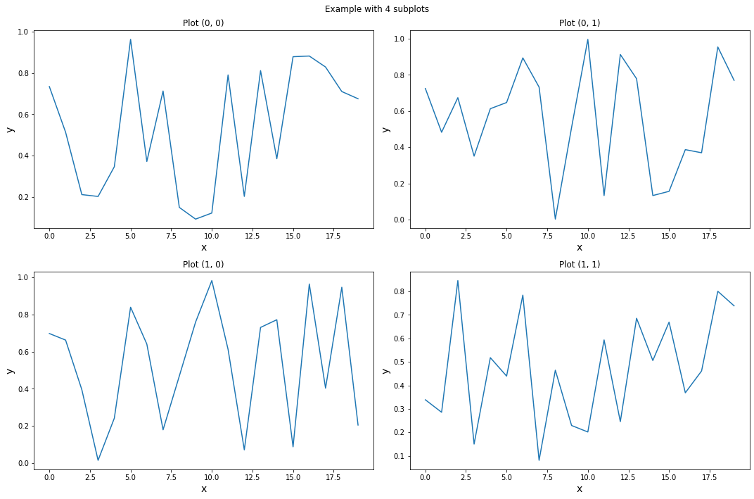
Seaborn is a library for making statistical graphics in Python.
It builds on top of matplotlib and integrates closely with pandas data structures.
It provides a high-level interface for drawing attractive and informative statistical graphics.
Its plotting functions operate on dataframes and arrays containing whole datasets and internally perform the necessary semantic mapping and statistical aggregation to produce informative plots.
Its dataset-oriented, declarative API lets you focus on what the different elements of your plots mean, rather than on the details of how to draw them.
For more see: https://seaborn.pydata.org/
Seaborn can be installed using either pip or Conda by running the following commands from the command line or Conda powershell.
python -m pip install seaborn
conda install seaborn
Seaborn is typically imported under the alias “sns”
# IMPORT SEABORN
import seaborn as sns
import matplotlib.pyplot as plt
Seaborn includes various sample data sets which can be used for educational purposes.
These are obtained using the “seaborn.load_dataset()” function which returns a dataset as a pandas data-frame.
The data is pulled from an online repository, therefore the function requires internet access to work.
A list of the available data sets can be found at the following link: https://github.com/mwaskom/seaborn-data
In the following examples, we will use the “tips” dataset which contains both continuous and categorical features.
It has 244 samples with seven features per sample, as showing in the following code cell.
# LOAD THE DATA-FRAME (REQUIRES INTERNET)
df = sns.load_dataset("tips")
print(df)
total_bill tip sex smoker day time size
0 16.99 1.01 Female No Sun Dinner 2
1 10.34 1.66 Male No Sun Dinner 3
2 21.01 3.50 Male No Sun Dinner 3
3 23.68 3.31 Male No Sun Dinner 2
4 24.59 3.61 Female No Sun Dinner 4
.. ... ... ... ... ... ... ...
239 29.03 5.92 Male No Sat Dinner 3
240 27.18 2.00 Female Yes Sat Dinner 2
241 22.67 2.00 Male Yes Sat Dinner 2
242 17.82 1.75 Male No Sat Dinner 2
243 18.78 3.00 Female No Thur Dinner 2
[244 rows x 7 columns]Seaborn has many different plotting commands. However, typically the syntax of the various commands is similar.
Below is a simple “scatterplot” example, where we plot two continuous numerical variables, one on the x-axis and the other on the y-axis.
sns.scatterplot(data=df, x="total_bill", y="tip")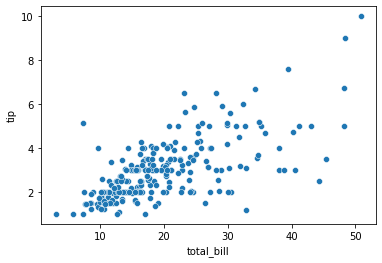
In data visualization, the term “encoding” describes the process of representing the variation in some numerical variable, either continuous or categorical, through aesthetic properties of the graph, such as size, shape, position, color, etc.
Seaborn makes encoding either continuous or categorical variables very easy.
The following is a list of some common encoding options in Seaborn.
However, different Seaborn commands have slightly different syntax.
Therefore they may require further googling to figure out the exact parameters.
data: “dataframe you want to plot”
x: “column of dataframe to use for x-axis”
y: “column of dataframe to use for y-axis”
col: “subplot option”
hue: “color encoding”
style: “marker encoding”
size: “size encoding’
In the previous example, we represented the continuous variables “tip” and “total_bill” using positional encodings along the x and y axis.
We can include additional information by specifying additional encodings, such as in the following example.
sns.scatterplot(data=df, x="total_bill", y="tip",size="size",hue="time", style="sex")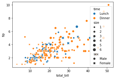
Notice that Seaborn automatically infers whether the variable is continuous or categorical, and then applies a logical encoding choice accordingly.
In the previous example the color encoding took on two distinct colors, because “time” is a binary categorical variable (Lunch or dinner).
However, in the following example the color is encoded in a continuously varying fashion, since “tip” is a continuous numeric variable.
sns.scatterplot(data=df, x="total_bill", y="tip",hue="tip")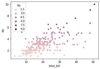
Seaborn is built on top of Matplotlib. Therefore, depending on the plotting command, it will return either a Matplotlib axes or figure object.
You can determine what is returned using the Python type() function
print(type(sns.scatterplot(data=df, x="total_bill", y="tip")))<class 'matplotlib.axes._subplots.AxesSubplot'>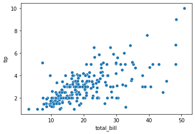
Notice, that the sns.scatterplot() function returns a MPL axes object. Therefore, we can use various MatplotLib axes commands to modify the Seaborn figure.
For example, in the next example we increase the figure (canvas) size by changing the MPL defaults in the rcParams dictionary.
Seaborn inherits various defaults from MPL, so this change will remain unless we change it back, or until you restart the python kernel, which will restore the un-modified defaults.
import matplotlib.pyplot as plt
plt.rcParams["figure.figsize"] = (10,10)
sns.scatterplot(data=df, x="total_bill", y="tip")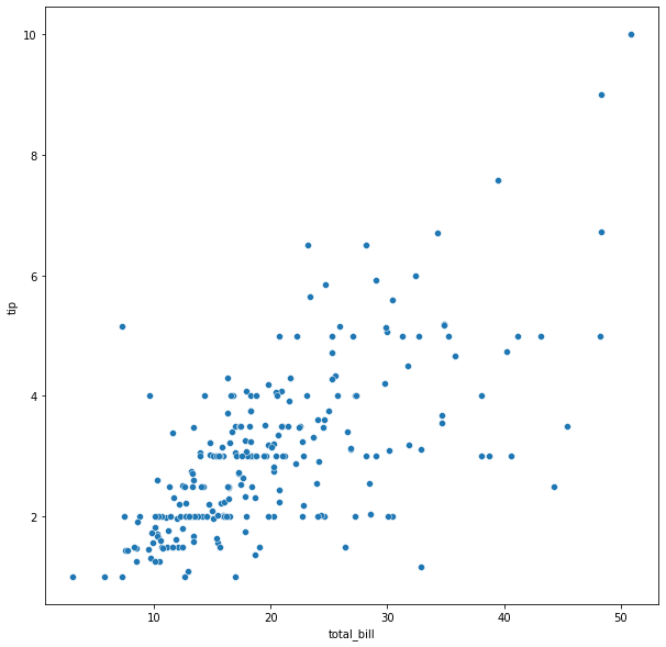
Typically the default axis-labels are un-acceptable for professional level presentations and plots. Since they are not very intelligible, lack units, and have font that is too small.
Therefore, we often want to modify them and increase the font size.
The following example compares a plot generated using the Seaborn defaults with one that is customized.
ax=sns.scatterplot(data=df, x="total_bill", y="tip", hue="time")
ax.set_title("EXAMPLE OF A BAD PLOT (WITH DEFAULTS)")
Text(0.5, 1.0, 'EXAMPLE OF A BAD PLOT (WITH DEFAULTS)')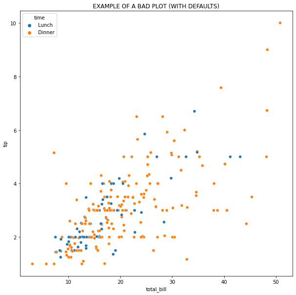
#NOTICE THAT "s" CONTROLS THE MARKER SIZE
ax=sns.scatterplot(data=df, x="total_bill", y="tip", s=200, hue="time")

ax.set_title("EXAMPLE OF A GOOD PLOT (WITH CUSTOMIZATION)",fontsize=20)

#LEGEND FONT SIZE
ax.legend(fontsize=20)

#AXIS LABELS AND FONT SIZE
ax.set_xlabel('Total bill at restaurant per table (US dollars)', fontsize=20)
ax.set_ylabel('Total tip per table (US dollars)', fontsize=20)

#AXIS TIC FONT SIZE
ax.tick_params(axis='both', which='major', labelsize=20)
ax.tick_params(axis='both', which='minor', labelsize=20)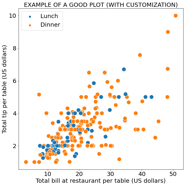
In some cases, Seaborn will return an object which is not a MLP axes or figure object.
my_plot=sns.relplot(
data=df,
x="total_bill",
y="tip",
col="time"
)
#NOTICE THE TYPES IS <class 'seaborn.axisgrid.FacetGrid'> NOT A MPL OBJECT
print(type(my_plot))
<class 'seaborn.axisgrid.FacetGrid'>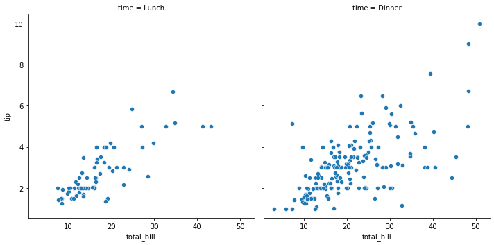
However, you can typically access the underline MLP objects via the attributes of the returned object, as shown in the following example.
g=sns.relplot(
data=df,
x="total_bill",
y="tip",
hue="sex",
col="time",
s=200,
)

#NOTICE THAT <class 'seaborn.axisgrid.FacetGrid'> OBJECT HAS ATTRIBUTES CONTAINING MPL OBJECTS
print('-----TYPES-----')
print(type(g.fig))
print(type(g.axes[0,0]))
print(type(g.axes[0,1]))

# BY ACCESSING THE MPL AXES/FIG ATTRIBUTES, WE CAN USE ALL OF OUR FAMILIAR MPL COMMANDS TO CUSTOMIZE

FS=16

#FIGURE TITLE
g.fig.set_size_inches(12, 6)

#AXIS LABELS AND FONT SIZE
g.axes[0,0].set_xlabel('Total bill at restaurant per table (US dollars)', fontsize=FS)
g.axes[0,0].set_ylabel('Total tip per table (US dollars)', fontsize=FS)

g.axes[0,1].set_xlabel('Total bill at restaurant per table (US dollars)', fontsize=FS)

#AXIS TIC FONT SIZE
for i in range(0,2):
    g.axes[0,i].tick_params(axis='both', which='major', labelsize=FS)
    #g.axes[0,i].tick_params(axis='both', which='minor', labelsize=FS)

#TITLE FONT SIZE
g.axes[0,0].set_title("Lunch time",fontsize=FS)
g.axes[0,1].set_title("Dinner time",fontsize=FS)

#LEGEND FONT SIZE
g.axes[0,0].legend(fontsize=FS)

#REMOVE SIDE LEGEND
g._legend.remove()
-----TYPES-----
<class 'matplotlib.figure.Figure'>
<class 'matplotlib.axes._subplots.AxesSubplot'>
<class 'matplotlib.axes._subplots.AxesSubplot'>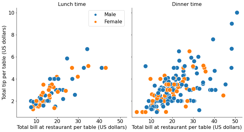
Seaborn includes various styles and color palettes for modifying the aesthetic of the plot.
The styles variable takes on four values; whitegrid, darkgrid, dark, and white.
The color palettes are the same as MPL, a description of them can be found at the following links * https://matplotlib.org/3.5.0/tutorials/colors/colormaps.html * https://seaborn.pydata.org/tutorial/color_palettes.html
The style and color palette can be modified individually using the following commands
sns.set_palette()sns.set_style()Or at the same time using the sns.set_theme() command, as shown in the following examples.
sns.set_theme(style='darkgrid', palette="Set2")
sns.scatterplot(data=df, x="total_bill", y="tip", hue="time")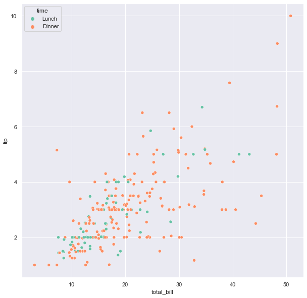
As mentioned above, the style and color palette can also be set individually, as in the following example.
As we can see, the result is identical to the previous example.
sns.set_palette(palette="Set2")
sns.set_style("darkgrid")
sns.scatterplot(data=df, x="total_bill", y="tip", hue="time")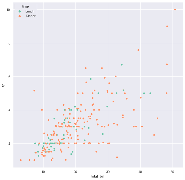
In the following examples, we explore the various styles along with different color palettes.
sns.set_theme(style='whitegrid', palette="Pastel1")
sns.scatterplot(data=df, x="total_bill", y="tip", hue="time")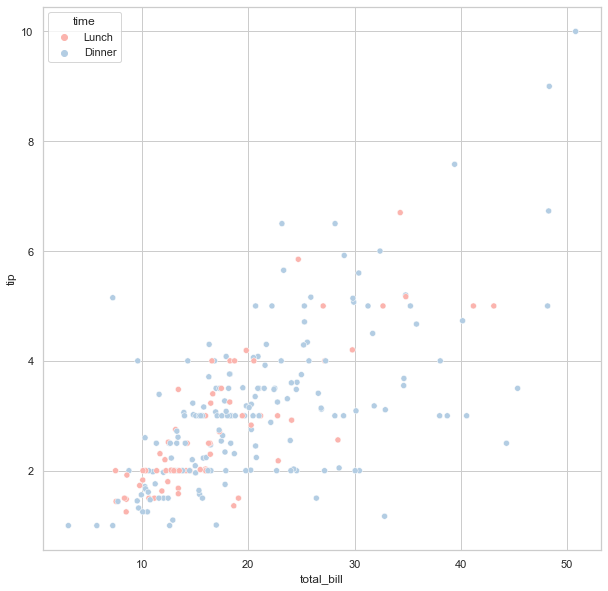
sns.set_theme(style='white', palette="husl")
sns.scatterplot(data=df, x="total_bill", y="tip", hue="time")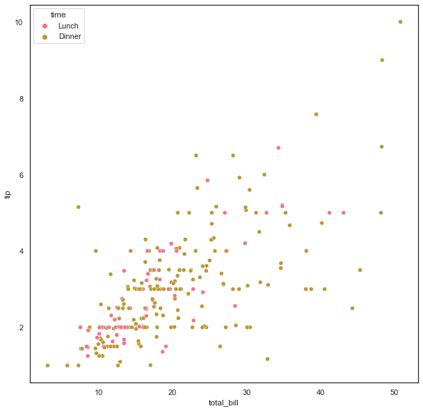
sns.set_theme(style='dark', palette="Set2")
sns.scatterplot(data=df, x="total_bill", y="tip", hue="time")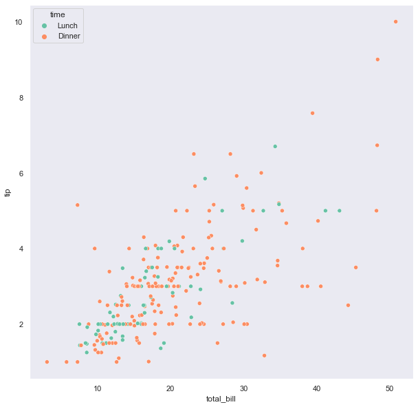
In the previous sections, we focused on the sns.scatterplot() function as an illustrative example.
However, there are many other Seaborn plotting functions.
The following standalone chunks of code are included as an example gallery.
The repeated import statements are included intentionally so that these codes could be copied and re-tooled in your own projects.
The examples below are just a small subset of what Seaborn can do. * For more examples see the following link * https://seaborn.pydata.org/examples/index.html
IMPORTANT NOTE: * In the examples below, we are using the Seaborn default values. * If we were planning to use these plots in a publication or project then we would need to do further customization to make them professionally acceptable.
import matplotlib.pyplot as plt
import seaborn  as sns

# LOAD AN EXAMPLE DATASET
df = sns.load_dataset("tips")
#print(df)

# RELPLOT
# This function provides access to several different
# axes-level functions that show the relationship between
# two variables with semantic mappings of subsets.
# The kind parameter selects the underlying axes-level
# function to use:
my_plot=sns.relplot(
    data=df,
    x="total_bill",
    y="tip",
    col="time",
    hue="smoker",
    style="smoker",
    size="size",
)

print(type(my_plot))
plt.show()
<class 'seaborn.axisgrid.FacetGrid'>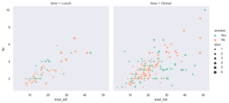
# LINEAR MODEL PLOT (lmplot --> Plot data and regression model fits across a FacetGrid)
sns.lmplot(
    data=df,
    x="total_bill",
    y="tip",
    col="time",
    hue="smoker")
print(type(my_plot))
plt.show()
<class 'seaborn.axisgrid.FacetGrid'>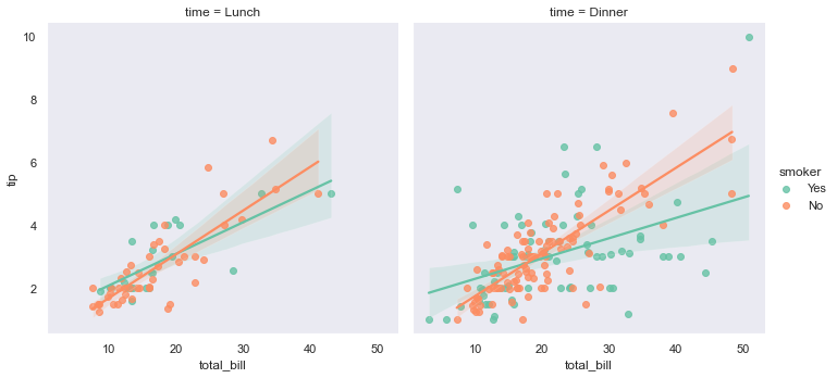
# DISTRIBUTION PLOT-1
sns.displot(
    data=df,
    x="total_bill",
    kde=True
    )
plt.show()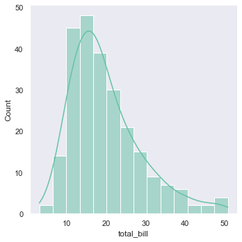
The “kde” option, stands for “kernel density estimation”.
KDE is a smoothing method used for estimating a continuous probability density distribution from a discrete histogram.
# DISTRIBUTION PLOT-2
sns.displot(
    data=df,
    x="total_bill",
    col="time",
    kde=True
    )
plt.show()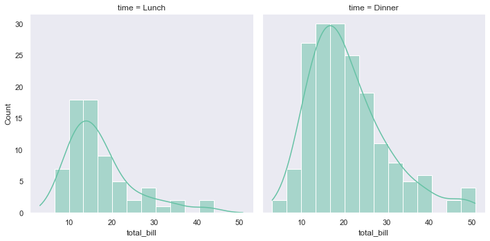
# CUMULATIVE DISTRIBUTION FUNCTION (CDF)

# Notice that we switch from a histogram (default) to a CDF using displot's kind="ecdf" option.
# Also, notice that we can introduce a rug plot, which shows each datapoint, projected on the X axis, using the "rug=True" option

sns.displot(
    data=df,
    kind="ecdf",
    x="total_bill",
    col="time",
    hue="smoker",
    rug=True
)
plt.show()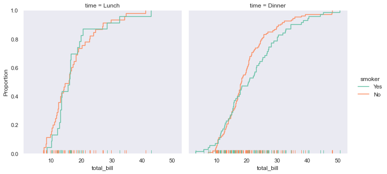
# SWARM PLOT-1
sns.catplot(
    data=df,
    kind="swarm",
    x="day",
    y="total_bill",
    hue="smoker")
plt.show()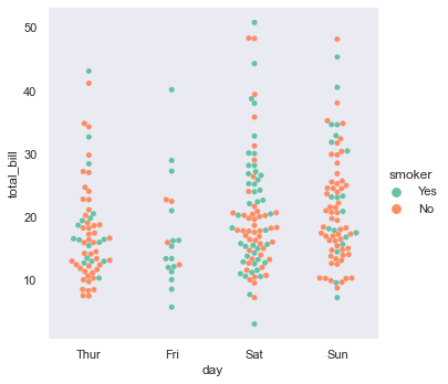
# VIOLIN PLOT
sns.catplot(
    data=df,
    kind="violin",
    x="day",
    y="total_bill",
    hue="smoker",
    split=True
)
plt.show()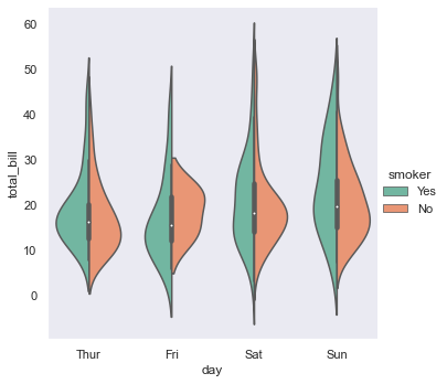
# BAR CHART
sns.catplot(
    data=df,
    kind="bar",
    x="day",
    y="total_bill",
    hue="smoker")
plt.show()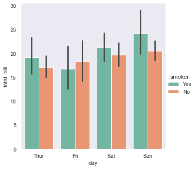
Disclaimer: This document is not an original work. It contains content from many sources and is for educational purposes only.
Sources: