import mathIntroduction to Numpy and Pandas
Packages
- Packages are an important tool that let us use existing code written by others (or ourselves) to accomplish high-level tasks.
- There are many packages available for Python, which is part of what makes it so powerful and popular.
- Packages are installed using a python “package manager”.
- They are typically installed in the
command lineterminal, using either thecondaorpippackage managers. For example:conda install numpypython -m pip install numpy
- Packages in python are simply a collection of one or more python
.pyfile(s).- When you install the package, these files are saved to your computer.
- You can then import the code from the packages into your own code and use them.
- This allows us to streamline our code by leveraging the work done by others, and avoid “reinventing the wheel”.
The import keyword
We can include the code from these packages using the import keyword. For example, let’s import the math package, which is already installed on our Base Python environment.
Now all the code from the math package is loaded into our working environment. From here, we can use functions and methods from this math package in our own code. Let’s use the factorial() function.
# print 5 factorial using the math package
print(math.factorial(5))120Note that we have to use the math package name before the function call. Otherwise, we will receive an error.
factorial(5)--------------------------------------------------------------------------- NameError Traceback (most recent call last) Cell In[3], line 1 ----> 1 factorial(5) NameError: name 'factorial' is not defined
Aliasing
Typing math before every function we want to use can become time-consuming and tedious. Instead, we can use aliasing to shorten the package name we write in our code. We use the as keyword to dictate we want to refer to the package using a different name in our code.
import math as mWe can then perform all the functions we want from the math packages but we will treat it as if it were just named m.
# print 5 factorial using the math package aliased as "m"
print(m.factorial(5))120Numpy
- Pandas
What is Numpy?
Numpyis a foundational package used by many data scientists and Python software developers for scientific computing.Its primary function is doing highly efficient linear algebra operations, similar to MATLAB.
- Because of this, it is the backbone of many other commonly used packages like
pandasandpyTorch.
- Because of this, it is the backbone of many other commonly used packages like
Numpy provides for the creation of multidimensional arrays (e.g. vectors, matrices, and tensors) objects that are abstract enough for virtually any task.
This package also provides functions for speedy operations on arrays ranging from simple matrix multiplication to discrete Fourier transformations.
Why Numpy?
Numpy is fast. In fact, code written with numpy would be way faster than if we were to implement the same code using Basic Python lists. As a short background, Python is written in C, one of the most efficient (and complicated) languages today. Even though it was created in the early 1970’s, it still remains common today for developers trying to achieve the most optimal and speedy code. The caveat here is that numpy is optimized to breakdown our code into C code at a faster rate than Base Python. Using this package certainly comes with some restrictions but the speed of this package much outweighs the limited freedoms. The Benchmark Comparison from The Computer Language Benchmarks Game shows just how fast C is compared to other common programming languages.
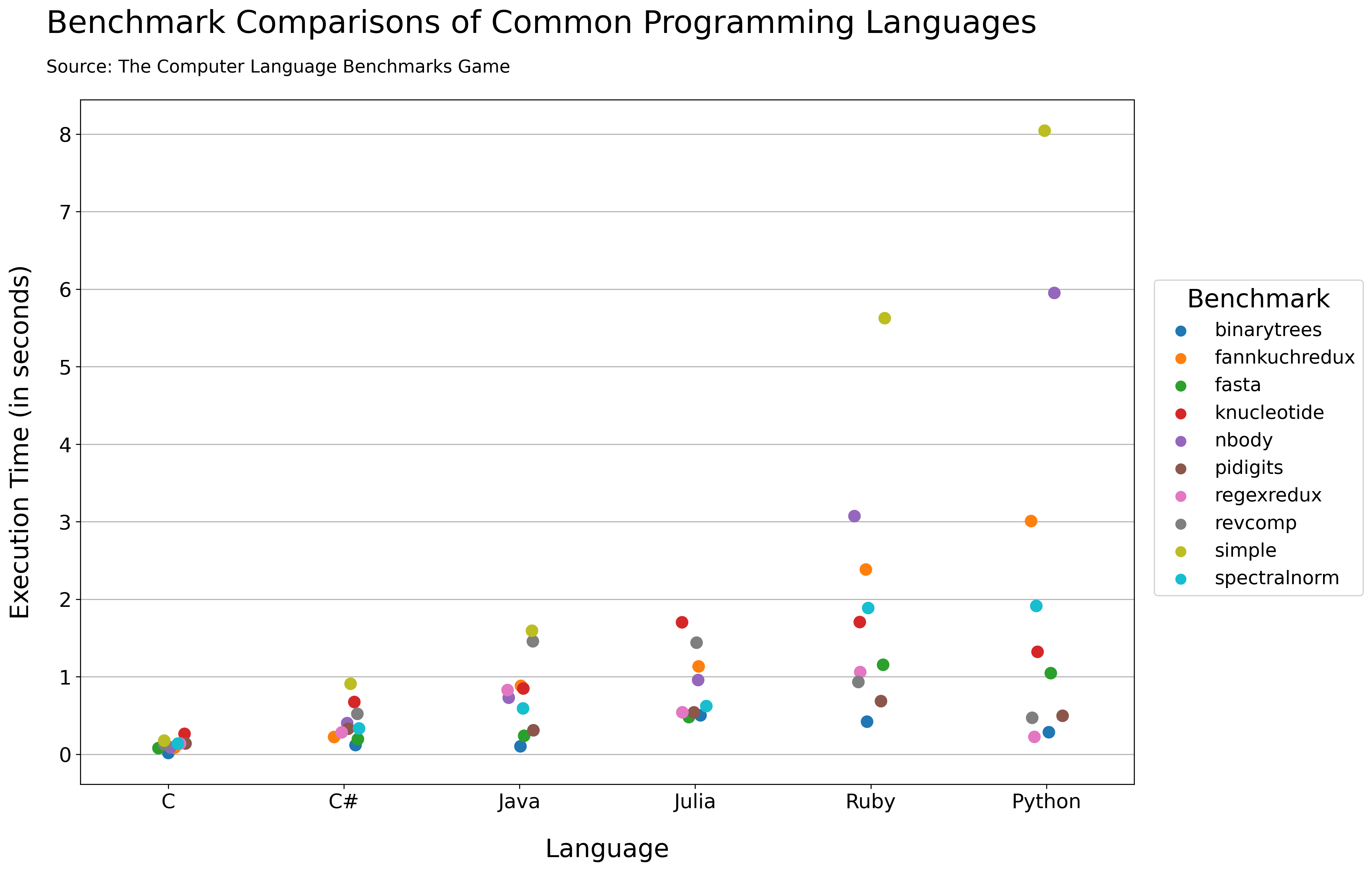
One other important, and highly efficient, computer language is Fortran. Similar to C, it is also popular in many computational science disciplines. However, due to its complexity, Fortran will not be discussed in this program.
Numpy leverages various important techniques from the field of high performance computing (HCP). This is the main reason it is so fast. These include concepts such as hyper-threading, vectorization, contiguous memory allocation, and the use of highly optimized linear algebra libraries such as BLAS and Intel’s math kernel library.
To prove that numpy is much faster than base Python methods, two scripts have been implemented below, one for Base Python and one for numpy. The overall goal is to compute the matrix multiplication of two \(200 \times 200\) matrices.
Base Python Matrix Multiplication
import numpy
import time  # this is another package that utilizes time-related functions

# save dimension as a variable
dims = 200

# create 2 random 200x200 matrices
matrix1 = [[numpy.random.randint(0,10) for i in range(dims)] for j in range(dims)]
matrix2 = [[numpy.random.randint(0,10) for i in range(dims)] for j in range(dims)]

# start the timer
baseStart = time.time()

# create a 200x200 matrix of zeros to hold the resulting matrix
myBaseMatrix = [[0]*dims]*dims

# matrix multiplication using base Python and for loops
for i in range(dims):
    for j in range(dims):
        for k in range(dims):
            myBaseMatrix[i][j] += matrix1[i][k] * matrix2[k][j]

# end the timer
baseEnd = time.time()

# substract the endtime from the start time
baseTime = baseEnd - baseStart
Numpy Matrix Multiplication
# save dimension as a variable
dims = 200

# create 2 random 200X200 matrices
matrix1 = numpy.random.randint(0,10, size = (dims,dims))
matrix2 = numpy.random.randint(0,10, size = (dims,dims))

# start the timer
numpyStart = time.time()

# Perform matrix multiplcation
myNumpyMatrix = numpy.matmul(matrix1,matrix2)

# end the timer
numpyEnd = time.time()

# substract the endtime from the start time
numpyTime = numpyEnd - numpyStart
Compare the Results
We see here that numpy blows our base Python algorithm out of the water. Hopefully, this shows just how important numpyis to data scientists and software developers.
# print the results
print(f'Base Python Time: {baseTime:.5f} microseconds')
print(f'Numpy Time: {numpyTime:.5f} microseconds')
print(f'\nNumpy is {baseTime/numpyTime:.3f} times as fast as Python')
Base Python Time: 2.55497 microseconds
Numpy Time: 0.01400 microseconds
Numpy is 182.505 times as fast as PythonArrays
First let’s import numpy. The common alias for this package is np as seen below.
import numpy as npCreation
Creating a numpy array from an existing Python list is relatively simple. We can use the np.array() function to transform a list. Another argument that can be used to specify the specific data type we want. For this implementation, we simply use "i" which is an integer that usually defaults to 32 or 64 bits or “memory” to store the number.
myList = [1,2,3,4,5,6]
myArray = np.array(myList, dtype = 'i')
print(myArray)
[1 2 3 4 5 6]Notice that this introduces a new data type to python (‘numpy.ndarray’). Similar to those discussed during week two.
print(type(myList))
print(type(myArray))
<class 'list'>
<class 'numpy.ndarray'>Dimensions
The ndim attribute of a Numpy array object tells us how many dimensions our data is. Since only a simple list was passed into the np.array() function, the array will have 1 dimension.
myArray.ndim1However, if we pass a 2-dimensional list, or a list of lists into the np.array() function, we will have created a matrix with rows and columns.
myList = [[1,2,3],[4,5,6]]
myArray = np.array(myList, dtype = 'i')
print(myArray)
[[1 2 3]
[4 5 6]]In this case, the dimensions of our array should be 2.
myArray.ndim2One of the notable restrictions in the numpy package is that our 2-dimensional list must be complete. If we pass in a list of lists where one list has 3 elements and another only has 2 elements, we get an error. Some exceptions in numpy can be confusing so be sure to check your bases when you are creating numpy arrays.
myList = [[1,2,3],[4,5]]   # PYthon list is not complete, will not work with numpy

myArray = np.array(myList, dtype = 'i')

print(myArray)
--------------------------------------------------------------------------- TypeError Traceback (most recent call last) TypeError: int() argument must be a string, a bytes-like object or a number, not 'list' The above exception was the direct cause of the following exception: ValueError Traceback (most recent call last) <ipython-input-15-09972e96b899> in <module> 1 myList = [[1,2,3],[4,5]] # PYthon list is not complete, will not work with numpy 2 ----> 3 myArray = np.array(myList, dtype = 'i') 4 5 print(myArray) ValueError: setting an array element with a sequence.
Shape
The shape is an important attribute of “numpy array” python objects. It is a tuple that tells us how many elements are in each dimension.
One dimensional arrays only require one index to specify a given site in the data structure. These are known as Numpy vectors.
myVector = np.array([4,5,6])
print(myVector)
print(myVector.shape)
print(myVector.ndim)
[4 5 6]
(3,)
1For 2-dimensional arrays (i.e. matrices), the shape corresponds to the number of rows and columns of the matrix.
myList = [[1,2,3],[4,5,6]]               # 2 dimensional python list
myArray = np.array(myList, dtype = 'i')

print(myArray, '\n')
print("2 ROWS AND 3 COLUMNS")
print(myArray.shape)
[[1 2 3]
[4 5 6]]
2 ROWS AND 3 COLUMNS
(2, 3)Notice that a vector can also be represented as a matrix, where one of its axes has length one.
#ROW VECTOR (1 ROW AND 3 COLUMNS )
myVector = np.array([[4,5,6]])
print(myVector)
print(myVector.shape)
print(myVector.ndim)
[[4 5 6]]
(1, 3)
2#COLUMN VECTOR (3 ROWS AND 1 COLUMN)
myVector = np.array([[4],[5],[6]])
print(myVector)
print(myVector.shape)
print(myVector.ndim)[[4]
[5]
[6]]
(3, 1)
2For higher dimensions (known as tensors), it can be harder to conceptualize (and visualize). However, the “shape” attribute will always be a tuple that has a length equal to the number of dimensions, ndim.
myList = [[[1,2],[3,4]],[[5,6],[7,8]]]  # 3 dimensional python list
myArray = np.array(myList, dtype = 'i')

print(myArray, '\n')
print(myArray.shape)
[[[1 2]
[3 4]]
[[5 6]
[7 8]]]
(2, 2, 2)This data structure is technically known as a rank three tensor, it can be visualized as a cube of data. Tensors with rank higher than three become impossible to visualize.
Data Type
The np.array object’s dtype attribute tells us what kind of data is stored in an array.
print(myArray.dtype)int32If we don’t specify the dtype argument when we create the array, numpy will usually find the best data type to use.
myList = [[1.0,2.0,3.0],[4,5,6]]
myArray = np.array(myList)
print(myArray, '\n')

print(myArray.dtype)
[[1. 2. 3.]
[4. 5. 6.]]
float64There are many dtypes that can be used but when creating an array, these will be the most common data types.
| Data Type | Default Size | Interpretation |
|---|---|---|
i |
32 bits | Integer |
b |
8 bits | Boolean |
uint |
32 bits | Unsigned Integer |
f |
64 bits | Floating Point Number |
M |
64 bits | DateTime |
O |
Depends on Input | Any Pythonic object |
S |
Depends on Input | String |
Abstract Creation
np.ones/np.zeros
Many times, we don’t want to explicitly define a numpy array using a list. The np.ones() and np.zeros() functions let us initialize an array of either 1's or 0's. By default, the data type of the created arrays are float64.
myArray = np.ones(6)

print(myArray, '\n')
print('ndims: ', myArray.ndim)
print('shape: ',myArray.shape)
print('dtype: ',myArray.dtype)
[1. 1. 1. 1. 1. 1.]
ndims: 1
shape: (6,)
dtype: float64We can also pass a shape argument into these functions, which must be a tuple defining the length of each dimension. In this case, we ask for 3 rows and 4 columns.
myArray = np.zeros(shape = (3,4))

print(myArray, '\n')
print('ndims: ', myArray.ndim)
print('shape: ',myArray.shape)
print('dtype: ',myArray.dtype)
[[0. 0. 0. 0.]
[0. 0. 0. 0.]
[0. 0. 0. 0.]]
ndims: 2
shape: (3, 4)
dtype: float64np.full
The np.full() function is similar to the np.ones() and np.zeros() function. However, it lets us choose what value to fill the array with. For this method, shape is the first argument of the function, and the fill_value argument dictates what value to fill the array with.
myArray = np.full(shape = (3,4), fill_value = 7)

print(myArray, '\n')
print('ndims: ', myArray.ndim)
print('shape: ',myArray.shape)
print('dtype: ',myArray.dtype)
[[7 7 7 7]
[7 7 7 7]
[7 7 7 7]]
ndims: 2
shape: (3, 4)
dtype: int32np.arange
The np.arange() function lets us make an array that contains values in a range. By default, if a single number is provided as an argument, it returns an array of integers starting at 0 and ending right before the number in the argument.
myArray = np.arange(8)

print(myArray, '\n')
print('ndims: ', myArray.ndim)
print('shape: ',myArray.shape)
print('dtype: ',myArray.dtype, '\n')
[0 1 2 3 4 5 6 7]
ndims: 1
shape: (8,)
dtype: int32
If we specify 2 arguments, then the values in the created array will start at the first argument and end right before the second argument. This is because Python is always inclusive on the left and exclusive on the right, as was described in week two.
myArray = np.arange(3,10)

print(myArray, '\n')
print('ndims: ', myArray.ndim)
print('shape: ',myArray.shape)
print('dtype: ',myArray.dtype, '\n')
[3 4 5 6 7 8 9]
ndims: 1
shape: (7,)
dtype: int32
Lets say we only want even numbers between 0 and 10. We can use a third argument, step, that tells numpy the step size to use. By default, the step size is 1.
myArray = np.arange(0,10, step = 2)

print(myArray, '\n')
print('ndims: ', myArray.ndim)
print('shape: ',myArray.shape)
print('dtype: ',myArray.dtype, '\n')
[0 2 4 6 8]
ndims: 1
shape: (5,)
dtype: int32
np.random.random
Numpy also has a random package inside. This package lets us create arrays with pseudo-random numbers. The np.random.random()function lets us make an array of a certain length, with numbers that are uniformly distributed between 0 and 1.
myArray = np.random.random(8)

print(myArray, '\n')
print('ndims: ', myArray.ndim)
print('shape: ',myArray.shape)
print('dtype: ',myArray.dtype)
[0.81772666 0.2709232 0.93851005 0.21763722 0.97388142 0.48873547
0.27544629 0.73570215]
ndims: 1
shape: (8,)
dtype: float64We can also create matrices or tensors by inputting a tuple.
myArray = np.random.random((2,3))
print(myArray)
[[0.86660377 0.44520249 0.07740186]
[0.49993227 0.26216785 0.48643139]]np.astype
Sometimes we may want to change the data type of our array (typecasting). This can be accomplished using the astype() function. Here we pass f into the dtype argument. The resulting array now has floating point number as its data type.
myArray = np.arange(8)

print(myArray, '\n')
print('ndims: ', myArray.ndim)
print('shape: ',myArray.shape)
print('dtype: ',myArray.dtype, '\n')

print("--Casting myArray to type float--\n")
myArray = myArray.astype(dtype = 'f')

print(myArray, '\n')
print('ndims: ', myArray.ndim)
print('shape: ',myArray.shape)
print('dtype: ',myArray.dtype)
[0 1 2 3 4 5 6 7]
ndims: 1
shape: (8,)
dtype: int32
--Casting myArray to type float--
[0. 1. 2. 3. 4. 5. 6. 7.]
ndims: 1
shape: (8,)
dtype: float32There are some considerations to keep in mind when changing the data type of an array. When we change the data type to a type that is less precise, we lose data. This is called downcasting. In the example below, we cast our floating point array as an integer array. In this case, we lose the decimal values.
myArray = np.array([3.14159,  2.71828])

print(myArray, '\n')
print('ndims: ', myArray.ndim)
print('shape: ',myArray.shape)
print('dtype: ',myArray.dtype, '\n')

print("--Casting myArray to type int--\n")
myArray = myArray.astype(dtype = 'i')

print(myArray, '\n')
print('ndims: ', myArray.ndim)
print('shape: ',myArray.shape)
print('dtype: ',myArray.dtype)
[3.14159 2.71828]
ndims: 1
shape: (2,)
dtype: float64
--Casting myArray to type int--
[3 2]
ndims: 1
shape: (2,)
dtype: int32Shaping
Shaping in numpy lets us changes the dimension and shape of our arrays without altering the elements within the array.
- Shaping operations are important in many applications including neural networks and deep learning.
np.reshape
The np.reshape() function lets us choose a new shape of our array.
- For example, we can reshape a 1-dimensional array with
9elements into a \(3\times 3\) array.
myArray = np.arange(9)

print(myArray, '\n')
print('ndims: ', myArray.ndim)
print('shape: ',myArray.shape)
print('dtype: ',myArray.dtype, '\n')

print("--Reshaping myArray to (3,3)--\n")
myArray = myArray.reshape(3,3)


print(myArray, '\n')
print('ndims: ', myArray.ndim)
print('shape: ',myArray.shape)
print('dtype: ',myArray.dtype, '\n')
[0 1 2 3 4 5 6 7 8]
ndims: 1
shape: (9,)
dtype: int32
--Reshaping myArray to (3,3)--
[[0 1 2]
[3 4 5]
[6 7 8]]
ndims: 2
shape: (3, 3)
dtype: int32
Note that the new shape that we define using the shape argument must be able to “fit” the array we are reshaping.
Consider what happens when we try to reshape a 1-dimensional array with 8 elements into a \(3\times 3\) array.
myArray = np.arange(8)

print(myArray, '\n')
print('ndims: ', myArray.ndim)
print('shape: ',myArray.shape)
print('dtype: ',myArray.dtype, '\n')

print("--Reshaping myArray to (3,3)--\n")
myArray = myArray.reshape(3,3)


print(myArray, '\n')
print('ndims: ', myArray.ndim)
print('shape: ',myArray.shape)
print('dtype: ',myArray.dtype, '\n')
[0 1 2 3 4 5 6 7]
ndims: 1
shape: (8,)
dtype: int32
--Reshaping myArray to (3,3)--
---------------------------------------------------------------------------
ValueError                                Traceback (most recent call last)
<ipython-input-34-7202baed8741> in <module>
      7
      8 print("--Reshaping myArray to (3,3)--\n")
----> 9 myArray = myArray.reshape(3,3)
     10
     11

ValueError: cannot reshape array of size 8 into shape (3,3)
Axis
In Numpy, the “axis” specifies which dimension you want to perform a specific operation across.
For example, whether you want to sum down the row (axis=0), or across the columns (axis=1).
myArray = np.array([[1,2,3],[4,5,6]])
print(myArray)
print("SUM DOWN THE ROWS (AXIS=0)")
print(myArray.sum(axis=0))
print("SUM ACROSS THE COLUMNS (AXIS=1)")
print(myArray.sum(axis=1))
[[1 2 3]
[4 5 6]]
SUM DOWN THE ROWS (AXIS=0)
[5 7 9]
SUM ACROSS THE COLUMNS (AXIS=1)
[ 6 15]np.concatenate
The np.concatenate() function lets us combine two arrays. Note that we must wrap the two arrays in a tuple or list for this function. The axis argument tells numpy which dimension to concatenate the arrays on. Since these arrays are only 1 dimension, we must call axis = 0.
a = np.arange(5)
b = np.arange(5)[::-1]


print('a:',a,a.shape)
print('b:',b,b.shape)

myConcatArray = np.concatenate( [a, b] ,  axis = 0)

print('\na + b =',myConcatArray)
a: [0 1 2 3 4] (5,)
b: [4 3 2 1 0] (5,)
a + b = [0 1 2 3 4 4 3 2 1 0]Concatenating multi-dimensional arrays can become more complex. Trying to concatenate two arrays on an incorrect axis will raise an error, and is a common error for both beginners and professionals. With more practice, it becomes easier to identify which axis to transform on.
a = np.arange(6).reshape(2,3)
b = np.arange(10).reshape(2,5)


print('a:\n',a,'\n')
print('b:\n',b)

#ACCROSS THE ROWS
myConcatArray = np.concatenate( [a, b] ,  axis = 1)

print('\na concatenated with b\n',myConcatArray)
a:
[[0 1 2]
[3 4 5]]
b:
[[0 1 2 3 4]
[5 6 7 8 9]]
a concatenated with b
[[0 1 2 0 1 2 3 4]
[3 4 5 5 6 7 8 9]]
a = np.arange(6).reshape(3,2)
b = np.arange(10).reshape(5,2)


print('a:\n',a,'\n')
print('b:\n',b)

#DOWN THE COLUMNS
myConcatArray = np.concatenate( [a, b] ,  axis = 0)

print('\na concatenated with b\n',myConcatArray)
a:
[[0 1]
[2 3]
[4 5]]
b:
[[0 1]
[2 3]
[4 5]
[6 7]
[8 9]]
a concatenated with b
[[0 1]
[2 3]
[4 5]
[0 1]
[2 3]
[4 5]
[6 7]
[8 9]]np.ravel/np.flatten
The np.ravel() and np.flatten() functions perform the exact same operation. They both turn a multi-dimensional array into a 1-dimensional array.
myArray = np.arange(9). reshape(3,3)

print(myArray, '\n')
print('ndims: ', myArray.ndim)
print('shape: ',myArray.shape)
print('dtype: ',myArray.dtype, '\n')


print('myArray.ravel():', myArray.ravel(), '\n')
print('myArray.flatten():', myArray.flatten())
[[0 1 2]
[3 4 5]
[6 7 8]]
ndims: 2
shape: (3, 3)
dtype: int32
myArray.ravel(): [0 1 2 3 4 5 6 7 8]
myArray.flatten(): [0 1 2 3 4 5 6 7 8]The only difference between these two methods is that np.ravel() generally returns a view while np.flatten() returns a copy.
The meaning of this will be discussed in more detail in the following sections.
Copies vs. Views
Whenever performing an operation on a numpy array and an array is returned, the array is either a view or a copy. A copy is relatively simple to understand. An entirely new portion of memory is allocated for this new array and all of the elements from the original array are copied to this new array. A view, however, is slightly more complex. When we create a view, the resulting array shares memory with the original array. This can get quite complicated but this means if we change the contents of the original array, the new array that is a view will also be affected by the change. The example below shows this phenomenon. A \(3\times 3\) array is created and a view is returned from using the np.ravel() function. One element in the original array is changed. It can be seen that this change also affects the view.
This may seem strange, however it can be very useful. Often when using large data (arrays), the amount of available computer memory (RAM) becomes a limitation.
Therefore, it is much more efficient to point to existing data in the memory rather than making a copy, which would waste memory space.
myOriginalArray = np.arange(9).reshape(3,3)

print('Original Array:\n', myOriginalArray, '\n')
print('ndims: ', myArray.ndim)
print('shape: ',myArray.shape)
print('dtype: ',myArray.dtype, '\n')

# use the ravel() function which returns a view
print("--Using ravel() function to create a view--\n")
myArrayView = myOriginalArray.ravel()

print('Array View:\n', myArrayView, '\n')
print('ndims: ', myArray.ndim)
print('shape: ',myArray.shape)
print('dtype: ',myArray.dtype, '\n')

# change the top left corner of the original matrix to 242
print("--Altering the Original Array--\n")
myOriginalArray[0,0] = 242

print('Original Array:\n', myOriginalArray, '\n')
print('ndims: ', myArray.ndim)
print('shape: ',myArray.shape)
print('dtype: ',myArray.dtype, '\n')

# print the array view to see that the data has changed
print('Array View:\n', myArrayView, '\n')
print('ndims: ', myArray.ndim)
print('shape: ',myArray.shape)
print('dtype: ',myArray.dtype, '\n')
Original Array:
[[0 1 2]
[3 4 5]
[6 7 8]]
ndims: 2
shape: (3, 3)
dtype: int32
--Using ravel() function to create a view--
Array View:
[0 1 2 3 4 5 6 7 8]
ndims: 2
shape: (3, 3)
dtype: int32
--Altering the Original Array--
Original Array:
[[242 1 2]
[ 3 4 5]
[ 6 7 8]]
ndims: 2
shape: (3, 3)
dtype: int32
Array View:
[242 1 2 3 4 5 6 7 8]
ndims: 2
shape: (3, 3)
dtype: int32
Even though we never altered myArrayView, it was still affected by changes performed on myOriginalArray.
np.copy
The np.copy() function can help mitigate some headaches when it comes to deciphering whether a returned array is a copy or a view. In the example, the new array is unaffected by changes in the original array.
myOriginalArray = np.arange(6)

print('Original Array:\n',myOriginalArray, '\n')
print('ndims: ', myArray.ndim)
print('shape: ',myArray.shape)
print('dtype: ',myArray.dtype, '\n')

# copy() the original array
print("--Using copy() function to create a copy--\n")
myArrayCopy = myOriginalArray.copy()

print('Copied Array:\n',myArrayCopy, '\n')
print('ndims: ', myArray.ndim)
print('shape: ',myArray.shape)
print('dtype: ',myArray.dtype, '\n')

# change the first element of the original matrix to 242
print("--Altering the Original Array--\n")
myOriginalArray[0] = 242

print('Original Array:\n',myOriginalArray, '\n')
print('ndims: ', myArray.ndim)
print('shape: ',myArray.shape)
print('dtype: ',myArray.dtype, '\n')

# print the array view to see that the data has changed
print('Copied Array:\n',myArrayCopy, '\n')
print('ndims: ', myArray.ndim)
print('shape: ',myArray.shape)
print('dtype: ',myArray.dtype, '\n')
Original Array:
[0 1 2 3 4 5]
ndims: 2
shape: (3, 3)
dtype: int32
--Using copy() function to create a copy--
Copied Array:
[0 1 2 3 4 5]
ndims: 2
shape: (3, 3)
dtype: int32
--Altering the Original Array--
Original Array:
[242 1 2 3 4 5]
ndims: 2
shape: (3, 3)
dtype: int32
Copied Array:
[0 1 2 3 4 5]
ndims: 2
shape: (3, 3)
dtype: int32
Transposition
Transposing an array is an important linear algebra operation.
The process of transposing in Numpy can be accomplished with the transpose() method function.
This creates a view of the original array that has a shape equal to the reverse of the original array’s shape.
a = np.zeros(shape = (1,2,3,4,5))
print("a.shape =",a.shape)

a_transpose = a.transpose()                      # the transpose is a view
print("\na_transpose.shape =",a_transpose.shape)
a.shape = (1, 2, 3, 4, 5)
a_transpose.shape = (5, 4, 3, 2, 1)In two dimensions, transposition can be interpreted and visualized as flipping the values of the array across the main diagonal of the array.
This means that the rows become the columns i.e. \(Transpose(A_{ij})=A_{ji}\).
a = np.arange(12).reshape(3,4)
print("a.shape =",a.shape)
print('a:\n',a)

a = a.transpose()                      # the transpose is a view
print("\na.shape =",a.shape)
print('a:\n',a)
a.shape = (3, 4)
a:
[[ 0 1 2 3]
[ 4 5 6 7]
[ 8 9 10 11]]
a.shape = (4, 3)
a:
[[ 0 4 8]
[ 1 5 9]
[ 2 6 10]
[ 3 7 11]]Mathematical Operations
Numpy also allows for a variety of numeric and logical operations on over two arrays.
These operations are performed element-wise, also known as component-wise.
This means that the resulting array from the operation is composed by performing the operation on each of element of one array with the corresponding element from another array.
\[ \]
\[\begin{bmatrix} 3 & 1 & 5 \\ 2 & 4 & 0 \\ 0 & 1 & 5 \end{bmatrix} + \begin{bmatrix} 2 & 2 & 1 \\ 3 & 0 & 1 \\ 0 & 2 & 4 \end{bmatrix} = \begin{bmatrix} 5 & 3 & 6 \\ 5 & 4 & 1 \\ 0 & 3 & 9 \end{bmatrix}\]
Numerical Operations
The following table shows a list of commonly used numerical operations for numpy arrays. These operations will always return a new array with a numeric data type.
| Algebraic Operator | numpy Operator | Sample condition | Interpretation |
|---|---|---|---|
| \(\times\) | * |
x * y |
x times y |
/ |
/ |
x / y |
x divided by y |
+ |
+ |
x + y |
x plus y |
- |
- |
x - y |
x minus y |
^ |
** |
x ** y |
x to the power of y |
mod |
% |
x % y |
x modulo y |
a = np.arange(1,7)
b = np.arange(1,7)[::-1]

print('a:\n', a, '\n')
print('b:\n', b, '\n')

print('\na + b:\n', a + b)
print('\na * b:\n', a * b)
print('\na ** b:\n', a ** b)
print('\na % b:\n', a % b)
a:
[1 2 3 4 5 6]
b:
[6 5 4 3 2 1]
a + b:
[7 7 7 7 7 7]
a * b:
[ 6 10 12 12 10 6]
a ** b:
[ 1 32 81 64 25 6]
a % b:
[1 2 3 1 1 0]Keep in mind that this element-wise operation property requires that our arrays have the same shape. Failing to ensure the two arrays have the same shape either results in a runtime error, where the code stops running, or a logical error, where the output array is not as expected.
a = np.arange(1,6)
b = np.arange(1,7)[::-1]

print("a.shape =",a.shape)
print('a:\n', a, '\n')

print("b.shape =",b.shape)
print('b:\n', b, '\n')

print('\na + b:\n', a + b)
a.shape = (5,)
a:
[1 2 3 4 5]
b.shape = (6,)
b:
[6 5 4 3 2 1]
---------------------------------------------------------------------------
ValueError                                Traceback (most recent call last)
<ipython-input-45-a8a9303a7655> in <module>
      8 print('b:\n', b, '\n')
      9
---> 10 print('\na + b:\n', a + b)

ValueError: operands could not be broadcast together with shapes (5,) (6,)
Logical Operations
The following table shows a list of commonly used logical operations for numpy arrays. These operations will always return a new array with the boolean data type.
| Algebraic Operator | numpy Operator | Sample condition | Interpretation |
|---|---|---|---|
| > | > |
x > y |
x is greater than y |
| < | < |
x < y |
x is less than y |
| ≥ | >= |
x >= y |
x is greater than or equal to y |
| ≤ | <= |
x <= y |
x is less than or equal to y |
| = | == |
x == y |
x is equal to y |
| ≠ | != |
x != y |
x is not equal to y |
a = np.arange(9).reshape(3,3)
b = np.arange(9)[::-1].reshape(3,3)

print('a:\n', a, '\n')
print('b:\n', b, '\n')

print('a < b:\n\n',a < b)
print('\na == b:\n\n',a == b)
a:
[[0 1 2]
[3 4 5]
[6 7 8]]
b:
[[8 7 6]
[5 4 3]
[2 1 0]]
a < b:
[[ True True True]
[ True False False]
[False False False]]
a == b:
[[False False False]
[False True False]
[False False False]]Broadcasting
Not all array operations have to use two arrays of the same shape. Broadcasting allows for us to implement some operations much easier.
Consider the case where we want multiply to each element of an array by 2. Certainly this example will get the job done.
a = np.arange(1,4)
print('a:\n',a)

b = np.full(3,2)
print('b:\n',b)

print('\na * b:\n',a * b)
a:
[1 2 3]
b:
[2 2 2]
a * b:
[2 4 6]If the shape of an array can be repeated and duplicated to fit the size of another array, we can use broadcasting to perform an operation on arrays of different sizes.
In the example below, 2 is treated as a \(1\times 1\) array and is stretched to fit the shape of a, which will result in an element-wise operation.
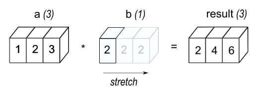 \[\text{Source: }\href{ https://numpy.org/doc/stable/user/basics.broadcasting.html}{numpy.org}\]
a = np.arange(1,4)
print('a:\n',a)

b = 2
print('\nb: ',b)

print('\na * b:\n',a * b)
a:
[1 2 3]
b: 2
a * b:
[2 4 6]Broadcasting Rules
Testing compatibility of two arrays for broadcasting can be summed up in 2 rules:
If two arrays don’t have the same number of dimensions, then the shape of the array with a lower number of dimensions is
prependedwith 1’s until the number of dimensions. Consider the following case.a.shape = (3,2,3) b.shape = (2,3)Because
bhas a lower number of dimensions thata, a 1 is prepended on the shape ofbuntil the number of dimensions matcha.shape = (3,2,3) b.shape = (1,2,3) <- 1 has been prepended to the shape of bArrays are compatible only if in each dimension one of these conditions are true:
the size of at least one of the dimensions is 1
the size of the dimensions are equal
  The following arrays are compatible
  a.shape = (2,3,3)
  b.shape = (1,3,3)

  The following arrays are NOT compatible
  a.shape = (2,3,3)
  b.shape = (1,3,4)
                 X   <- Last dimensions are not equal and neither of them are 1
More Examples
We can get more complex with this concept. We can add an array of length \(3\) to a \(4\times 3\) array. Let’s check for compatibility.
- The number of the dimensions are not the same for both arrays
- prepend a 1 to the shape of smaller array, it is now a \(1 \times 3\) array
- In the first dimension, at least one of them dimensions has a size of 1
- In the second dimension, the sizes of the dimensions are equal
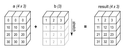 \[\text{Source: }\href{ https://numpy.org/doc/stable/user/basics.broadcasting.html}{numpy.org}\]
a = np.array([[ 0.0,  0.0,  0.0],
           [10.0, 10.0, 10.0],
           [20.0, 20.0, 20.0],
           [30.0, 30.0, 30.0]])
print("a.shape =",a.shape)
print('a:\n',a)

b = np.arange(1,4)
print("\nb.shape =",b.shape)
print('b:\n',b)

print('\na + b:\n',a + b)
a.shape = (4, 3)
a:
[[ 0. 0. 0.]
[10. 10. 10.]
[20. 20. 20.]
[30. 30. 30.]]
b.shape = (3,)
b:
[1 2 3]
a + b:
[[ 1. 2. 3.]
[11. 12. 13.]
[21. 22. 23.]
[31. 32. 33.]]However, we can’t add an array of length \(4\) to a \(4\times 3\) array. Let’s check for compatibility and see why.
- The number of the dimensions are not the same for both arrays
- prepend a 1 to the shape of smaller array, it is now a \(1 \times 4\) array
- In the first dimension, at least one of them dimensions has a size of 1
- In the second dimension, the sizes of the dimensions are NOT equal nor does at least one of them have a size of 1
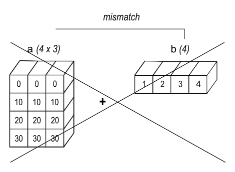 \[\text{Source: }\href{ https://numpy.org/doc/stable/user/basics.broadcasting.html}{numpy.org}\]
a = np.array([[ 0.0,  0.0,  0.0],
           [10.0, 10.0, 10.0],
           [20.0, 20.0, 20.0],
           [30.0, 30.0, 30.0]])
print("a.shape =",a.shape)
print('a:\n',a)

b = np.arange(1,5)
print("\nb.shape =",b.shape)
print('b:\n',b)

print('\na + b:\n',a + b)
a.shape = (4, 3)
a:
[[ 0. 0. 0.]
[10. 10. 10.]
[20. 20. 20.]
[30. 30. 30.]]
b.shape = (4,)
b:
[1 2 3 4]--------------------------------------------------------------------------- ValueError Traceback (most recent call last) <ipython-input-50-34135da6caf7> in <module> 10 print('b:\n',b) 11 ---> 12 print('\na + b:\n',a + b) ValueError: operands could not be broadcast together with shapes (4,3) (4,)
Let’s try to add an array of length \(3\) to a \(4\times 1\) array. Let’s check for compatibility.
- The number of the dimensions are not the same for both arrays
- prepend a 1 to the shape of smaller array, it is now a \(1 \times 3\) array
- In the first dimension, at least one of them dimensions has a size of 1
- In the second dimension, at least one of them dimensions has a size of 1
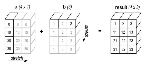 \[\text{Source: }\href{ https://numpy.org/doc/stable/user/basics.broadcasting.html}{numpy.org}\]
a = np.arange(0,40,10).reshape(4,1)
print("a.shape =",a.shape)
print('a:\n',a)

b = np.arange(1,4)
print("\nb.shape =",b.shape)
print('b:\n',b)

print('\na + b:\n',a + b)
a.shape = (4, 1)
a:
[[ 0]
[10]
[20]
[30]]
b.shape = (3,)
b:
[1 2 3]
a + b:
[[ 1 2 3]
[11 12 13]
[21 22 23]
[31 32 33]]Upcasting
You may have noticed earlier that when we created an array from a list that contained both integers and floating point numbers, the resulting array had a float64 data type. Numpy noticed that the data types in the list did not match and performed what is called upcasting. Whenever a situation like this occurs, numpy will always choose the most precise data type and cast each element as that data type. Because floating point numbers are more precise than integers, the integers were cast as floating point numbers.
myList = [[1.0, 2.0, 3.0],[4, 5, 6]]
a = np.array(myList)

print(a, '\n')
print(a.dtype)
[[1. 2. 3.]
[4. 5. 6.]]
float64Upcasting also occurs when performing numerical operations.
a = np.arange(6)
b = np.random.random(6)

print('a:\n', a, '\n')
print('a Data Type:', a.dtype, '\n')

print('b:\n', b, '\n')
print('b Data Type:\n', b.dtype, '\n')


NewArray = a + b
print('a:\n', NewArray, '\n')
print('a + b Data Type:', NewArray.dtype, '\n')
a:
[0 1 2 3 4 5]
a Data Type: int32
b:
[0.98763621 0.00743969 0.5607724 0.62347624 0.35429875 0.71658622]
b Data Type:
float64
a:
[0.98763621 1.00743969 2.5607724 3.62347624 4.35429875 5.71658622]
a + b Data Type: float64
Universal Functions
Universal Functions, or ufuncs, are functions that be applied element-wise on an array. The following table describes some common ufuncs.
| ufunc | Interpretation |
|---|---|
np.exp |
Natural Exponentiation |
np.sqrt |
Square Root |
np.sin |
Sine |
np.cos |
Cosine |
np.log |
Natural Logarithm |
np.isinf |
Check For Infinity |
a = np.arange(1,6)

print('a:\n', a, '\n')

print('np.exp(a):\n', np.exp(a), '\n')
print('np.sqrt(a):\n', np.sqrt(a), '\n')
print('np.log(a):\n', np.log(a), '\n')
print('np.isinf(a):\n', np.isinf(a), '\n')
a:
[1 2 3 4 5]
np.exp(a):
[ 2.71828183 7.3890561 20.08553692 54.59815003 148.4131591 ]
np.sqrt(a):
[1. 1.41421356 1.73205081 2. 2.23606798]
np.log(a):
[0. 0.69314718 1.09861229 1.38629436 1.60943791]
np.isinf(a):
[False False False False False]
Indexing
Indexing is a very important skill to learn when using numpy. The syntax resembles that of Python but comes with some new features. These examples will be implemented on a 2-dimensional array but follows the same logic for higher-dimensional arrays.
a = np.arange(16).reshape(4,4)
print(a)
[[ 0 1 2 3]
[ 4 5 6 7]
[ 8 9 10 11]
[12 13 14 15]]Indexing uses each axis as a reference. To index the first row of a multidimensional array, we index as we normally do in base Python.
print(a[0])[0 1 2 3]To index a specific element, we use more than one index, separated by a comma. This example tells numpy to look at index 0 in the rows dimension and to look at index 2 in the column dimension.
print(a[0,2])2To index the first column of a multidimensional array, we use the : operator and a comma. This is telling numpy to look at every row but only index the first element of each row.
print(a[:,0])[ 0 4 8 12]Therefore, using the : operator for the first and second axis dimensions tells numpy to extract every row and every column. yielding a view of the original array. Note that all indexing operations will return a view rather than copy.
print(a[:,:])[[ 0 1 2 3]
[ 4 5 6 7]
[ 8 9 10 11]
[12 13 14 15]]Because this array is only 2 dimensions. We cannot index any more than 2 dimensions. Doing so will yield an error.
print(a[2,:,:])--------------------------------------------------------------------------- IndexError Traceback (most recent call last) <ipython-input-60-1d4a5b2adc8c> in <module> ----> 1 print(a[2,:,:]) IndexError: too many indices for array: array is 2-dimensional, but 3 were indexed
We can also use ranges while indexes. This example tells numpy that we want the first 2 rows and every column.
print(a[0:2, :])[[0 1 2 3]
[4 5 6 7]]We can use ranges in multiple dimensions when indexing. This example tells numpy that we want the first 2 rows and the first 3 columns.
a[0:2,0:3]array([[0, 1, 2],
[4, 5, 6]])We can index a row out of a numpy array, then index that row itself. Operations like this are not exclusive to indexing or numpy and is called chaining.
print(a[0])[0 1 2 3]print(a[0][0])0# some index chaining
print(a[:,:3][:2,:][1][2])6Pandas
- Pandas
Introduction
Pandas is a package built on top of numpy that excels at manipulating and cleaning data. There are two major objects that can be created with Pandas:
- Series
- Can be thought of as a “column” of data
- Comparable to a
numpyarray object - All entries in a Series must have the same data type
- DataFrame
- A rectangular dataset
- Has columns and rows of data
- Can hold heterogeneous data between columns
- It a container that is collection of Series objects
Aliasing
Pandas is commonly aliased as pd
import pandas as pdCreating A Series
To create a Series object, the pandas.Series() function needs to be called. The argument for this function can be many data structures, but lists and dictionaries are used the most.
s = pd.Series(["Sayonara", "Racecar", "Carousel", "Pony"])  # call the Series function with a list

print(s)
0 Sayonara
1 Racecar
2    Carousel
3        Pony
dtype: objectIndex and Slicing a Series
On the left side of the printed Series are the row numbers. This acts as the index for a Series. Indexing and Slicing from numpy can be applied here. If more than one element is extracting from slicing, then a view of the Series is returned.
print(s[1]) # index the element in the Series at index 1Racecarprint(s[2:4]) # index the elements from index 2 up to but not including index 42 Carousel
3 Pony
dtype: objectYou can also use a list of index values to slice a Series.
indexes = [0,1,3]

print(s[indexes])
0 Sayonara
1 Racecar
3 Pony
dtype: objectThe index of Series objects can be changed as well. The values of the indexes do not have to be unique.
s = pd.Series(
    data = ["Sayonara", "Racecar", "Carousel", "Pony"],
    index = ["Song 1", "Song 2", "Song 3","Song 4"])  # create a custom index,

print(s)
Song 1 Sayonara
Song 2     Racecar
Song 3    Carousel
Song 4        Pony
dtype: objectThese custom indexes can be useful to index the Series in another way
print(s["Song 4"]) # index the element in the series with the index "Song 4"PonyHowever, it is still possible to index a Series using the traditional numpy slicing techniques.
print(s[1:4]) # index the elements from index 1 up to but not including index 4Song 2 Racecar
Song 3 Carousel
Song 4 Pony
dtype: objectCreating a Dataframe
Dataframes are an ordered collection of Series. The words column or Series are used interchangeably when referring to a vertical column in a DataFrame. To create a DataFrame object, the pandas.DataFrame() function needs to be called. The argument for this function is generally a numpy array or a Python dictionary. Initialized Dataframes are commonly assigned the name df.
# create a dataframe
df = pd.DataFrame({
    'Name': ['Rosaline Franklin', 'William Gosset'],
    'Occupation': ['Chemist', 'Statistician'],
    'Born': ['1920-07-25', '1876-06-13'],
    'Died': ['1958-04-16', '1937-10-16'],
    'Age': [37, 61]},
    index = ["Index 1", "Index 2"])

print(df)
Name Occupation Born Died Age
Index 1 Rosaline Franklin Chemist 1920-07-25 1958-04-16 37
Index 2 William Gosset Statistician 1876-06-13 1937-10-16 61Attributes
Shape
Similar to numpy arrays, the shape attribute tells us the length of the rows and columns of a DataFrame.
print(df.shape)

print("\nNumber of Rows:", df.shape[0])
print("Number of Columns:", df.shape[1])
(2, 5)
Number of Rows: 2
Number of Columns: 5Columns
The columns attribute returns a list-like object of the column names of the DataFrame.
print(df.columns)Index(['Name', 'Occupation', 'Born', 'Died', 'Age'], dtype='object')Index
Similarly, the index attribute returns a list-like object of the index names or row names of the DataFrame.
print(df.index)Index(['Index 1', 'Index 2'], dtype='object')Slicing a DataFrame
Slicing DataFrames can have a slightly different syntax than Series.
Slicing a Column
To extract a single column from a DataFrame, you can use the column name wrapped in square brackets.
print(df["Name"])Index 1 Rosaline Franklin
Index 2 William Gosset
Name: Name, dtype: objectprint(df["Age"])Index 1 37
Index 2 61
Name: Age, dtype: int64To extract more than one column from a DataFrame, use a list of column names.
cols = ["Occupation", "Died", "Age"] # list of column names

print(df[cols])
Occupation Died Age
Index 1 Chemist 1958-04-16 37
Index 2 Statistician 1937-10-16 61Slicing a Row
There are two methods to slice a row: * pandas.iloc : Slices the Dataframe by the row position index * pandas.loc : Slices the Dataframe by the name of the Index
Notice that the row that is extracted from the DataFrame is also a Series.
print(df.iloc[0]) # this will extract the first row of the dataframe, regardless of index nameName Rosaline Franklin
Occupation Chemist
Born 1920-07-25
Died 1958-04-16
Age 37
Name: Index 1, dtype: objectprint(df.loc["Index 1"]) # this will extract the row or rows named "Index 1"Name Rosaline Franklin
Occupation Chemist
Born 1920-07-25
Died 1958-04-16
Age 37
Name: Index 1, dtype: objectExtracting a Single Data Point
pandas.loc and pandas.iloc can also be used to extract single pieces of data.
- pandas.iloc[ ROW_INDEX, COLUMN_INDEX]
- pandas.loc[ ROW_NAME, COLUMN_NAME]
print(df.iloc[0,1]) # extract first row and second column of the dataframe, regardless of index or column nameChemistprint(df.loc["Index 1", "Born"]) # extract the row or rows named "Index 1" and the column named "Born"1920-07-25Extracting More Than One Data Point
Using the pandas.iloc function and lists of column and row indices, you can slice a dataframe however you choose.
cols = [1, 3, 4]     # list of column indices
inds = [0, 1]        # List of row indices

print(df.iloc[inds, cols])
Occupation Died Age
Index 1 Chemist 1958-04-16 37
Index 2 Statistician 1937-10-16 61Additionally, by using the pandas.loc function and lists of column and row names, you can slice a dataframe however you choose and accomplish the same task.
cols = ["Occupation", "Died", "Age"] # list of column names
inds = ["Index 1", "Index 2"]        # List of index names

print(df.loc[inds, cols])
Occupation Died Age
Index 1 Chemist 1958-04-16 37
Index 2 Statistician 1937-10-16 61Reading In Data
Often, we want to read in a dataset from a file. Pandas has functions that make this process easy for us.
The pandas.read_csv function
One of the most common file types for storing data is a .csv file. The read_csv() function will read in a .csv file and store it as a DataFrame.
#                 FILE LOCATION
iris = pd.read_csv("./iris.csv")

# print the dataframe
print(iris)
sepal.length sepal.width petal.length petal.width variety
0 5.1 3.5 1.4 0.2 Setosa
1 4.9 3.0 1.4 0.2 Setosa
2 4.7 3.2 1.3 0.2 Setosa
3 4.6 3.1 1.5 0.2 Setosa
4 5.0 3.6 1.4 0.2 Setosa
.. ... ... ... ... ...
145 6.7 3.0 5.2 2.3 Virginica
146 6.3 2.5 5.0 1.9 Virginica
147 6.5 3.0 5.2 2.0 Virginica
148 6.2 3.4 5.4 2.3 Virginica
149 5.9 3.0 5.1 1.8 Virginica
[150 rows x 5 columns]header argument
If the dataset you are trying to read in does not have any column names, make use of the header argument in the function declaration. This will tell pandas that the file does not have any column names. Let’s demonstrate this example on the iris.csv dataset. Because this data does have column names, the first entry in the dataset at index 0 are the column names. While this should not be done in practice, it does demonstrate the utility of the header argument.
#                    FILE LOCATION       # Use if dataset has no column names
iris = pd.read_csv(   "./iris.csv"   ,     header = None)

# print dataset
print(iris) # because this dataset has column names, the column names will be rows
0 1 2 3 4
0 sepal.length sepal.width petal.length petal.width variety
1 5.1 3.5 1.4 .2 Setosa
2 4.9 3 1.4 .2 Setosa
3 4.7 3.2 1.3 .2 Setosa
4 4.6 3.1 1.5 .2 Setosa
.. ... ... ... ... ...
146 6.7 3 5.2 2.3 Virginica
147 6.3 2.5 5 1.9 Virginica
148 6.5 3 5.2 2 Virginica
149 6.2 3.4 5.4 2.3 Virginica
150 5.9 3 5.1 1.8 Virginica
[151 rows x 5 columns]To correct this error, let’s reassign the iris variable so that the DataFrame has headers.
#                 FILE LOCATION
iris = pd.read_csv("./iris.csv")
While the function is called read_csv, it has more uses than just reading in Comma Separated Value (CSV) files. It can read in any character delimited file, like Tab Separated Value (TSV) files.
Let’s read in the gapminder.tsv file. Because this file separates the values using a tab rather than a comma, we have to declare the delimiter argument as \t which is the escape character for a tab.
#                         FILE LOCATION    DELIMITER SET TO TAB
Gapminder = pd.read_csv('./gapminder.tsv', delimiter= '\t')
The pandas.read_json function
Another popular file type for storing data is a .json file. These files look like large nested Python dictionaries. A truncated version of the Advertising.json file is shown below.
{ <- Outer Dictionary
“TV”: { <- Inner Dictionary
“0”: 230.1,
“1”: 44.5,
…
“198”: 283.6,
“199”: 232.1
},
“Radio”: { <- Inner Dictionary
“0”: 37.8,
“1”: 39.3,
…
“198”: 42,
“199”: 8.6
},
“Newspaper”: { <- Inner Dictionary
“0”: 69.2,
“1”: 45.1,
…
“198”: 66.2,
“199”: 8.7
},
“Sales”: { <- Inner Dictionary
“0”: 22.1,
“1”: 10.4,
…
“198”: 25.5,
“199”: 13.4
}
}
To read in a .json file, simply use the read_json() function.
#                             FILE LOCATION
Advertising = pd.read_json("./Advertising.json")


print(Advertising)
TV Radio Newspaper Sales
0 230.1 37.8 69.2 22.1
1 44.5 39.3 45.1 10.4
2 17.2 45.9 69.3 9.3
3 151.5 41.3 58.5 18.5
4 180.8 10.8 58.4 12.9
.. ... ... ... ...
195 38.2 3.7 13.8 7.6
196 94.2 4.9 8.1 9.7
197 177.0 9.3 6.4 12.8
198 283.6 42.0 66.2 25.5
199 232.1 8.6 8.7 13.4
[200 rows x 4 columns]Looking At Data
Next, let’s look at some methods to look at our data. You have already seen the print method, which generally prints the first 5 and last 5 entries in the dataframe.
# print the dataset
print(Gapminder)
country continent year lifeExp pop gdpPercap
0 Afghanistan Asia 1952 28.801 8425333 779.445314
1 Afghanistan Asia 1957 30.332 9240934 820.853030
2 Afghanistan Asia 1962 31.997 10267083 853.100710
3 Afghanistan Asia 1967 34.020 11537966 836.197138
4 Afghanistan Asia 1972 36.088 13079460 739.981106
... ... ... ... ... ... ...
1699 Zimbabwe Africa 1987 62.351 9216418 706.157306
1700 Zimbabwe Africa 1992 60.377 10704340 693.420786
1701 Zimbabwe Africa 1997 46.809 11404948 792.449960
1702 Zimbabwe Africa 2002 39.989 11926563 672.038623
1703 Zimbabwe Africa 2007 43.487 12311143 469.709298
[1704 rows x 6 columns]head
The head() method function returns the first 5 entries in the DataFrame.
# print the first 5 entries of the dataframe
print(Gapminder.head())
country continent year lifeExp pop gdpPercap
0 Afghanistan Asia 1952 28.801 8425333 779.445314
1 Afghanistan Asia 1957 30.332 9240934 820.853030
2 Afghanistan Asia 1962 31.997 10267083 853.100710
3 Afghanistan Asia 1967 34.020 11537966 836.197138
4 Afghanistan Asia 1972 36.088 13079460 739.981106If we add a number as an argument to the head() method function, it will return that many entries from the beginning of the DataFrame.
# print the first 10 entries of the dataframe
print(Gapminder.head(10))
country continent year lifeExp pop gdpPercap
0 Afghanistan Asia 1952 28.801 8425333 779.445314
1 Afghanistan Asia 1957 30.332 9240934 820.853030
2 Afghanistan Asia 1962 31.997 10267083 853.100710
3 Afghanistan Asia 1967 34.020 11537966 836.197138
4 Afghanistan Asia 1972 36.088 13079460 739.981106
5 Afghanistan Asia 1977 38.438 14880372 786.113360
6 Afghanistan Asia 1982 39.854 12881816 978.011439
7 Afghanistan Asia 1987 40.822 13867957 852.395945
8 Afghanistan Asia 1992 41.674 16317921 649.341395
9 Afghanistan Asia 1997 41.763 22227415 635.341351tail
The tail() method function will return the last 5 entries from a DataFrame.
# print the last 5 entries of the dataframe
print(Gapminder.tail())
country continent year lifeExp pop gdpPercap
1699 Zimbabwe Africa 1987 62.351 9216418 706.157306
1700 Zimbabwe Africa 1992 60.377 10704340 693.420786
1701 Zimbabwe Africa 1997 46.809 11404948 792.449960
1702 Zimbabwe Africa 2002 39.989 11926563 672.038623
1703 Zimbabwe Africa 2007 43.487 12311143 469.709298Similarly, if we add a number as an argument to the tail() method function, it will return that many entries from the end of the DataFrame.
# print the last 8 entries of the dataframe
print(Gapminder.tail(8))
country continent year lifeExp pop gdpPercap
1696 Zimbabwe Africa 1972 55.635 5861135 799.362176
1697 Zimbabwe Africa 1977 57.674 6642107 685.587682
1698 Zimbabwe Africa 1982 60.363 7636524 788.855041
1699 Zimbabwe Africa 1987 62.351 9216418 706.157306
1700 Zimbabwe Africa 1992 60.377 10704340 693.420786
1701 Zimbabwe Africa 1997 46.809 11404948 792.449960
1702 Zimbabwe Africa 2002 39.989 11926563 672.038623
1703 Zimbabwe Africa 2007 43.487 12311143 469.709298describe
The describe() method function will return descriptive statistics on each of the numerical columns of the DataFrame.
print(Gapminder.describe()) year lifeExp pop gdpPercap
count 1704.00000 1704.000000 1.704000e+03 1704.000000
mean 1979.50000 59.474439 2.960121e+07 7215.327081
std 17.26533 12.917107 1.061579e+08 9857.454543
min 1952.00000 23.599000 6.001100e+04 241.165877
25% 1965.75000 48.198000 2.793664e+06 1202.060309
50% 1979.50000 60.712500 7.023596e+06 3531.846989
75% 1993.25000 70.845500 1.958522e+07 9325.462346
max 2007.00000 82.603000 1.318683e+09 113523.132900info
The info() method function will return a summary of each of the columns including their data type.
print(Gapminder.info()) <class 'pandas.core.frame.DataFrame'>
RangeIndex: 1704 entries, 0 to 1703
Data columns (total 6 columns):
# Column Non-Null Count Dtype
--- ------ -------------- -----
0 country 1704 non-null object
1 continent 1704 non-null object
2 year 1704 non-null int64
3 lifeExp 1704 non-null float64
4 pop 1704 non-null int64
5 gdpPercap 1704 non-null float64
dtypes: float64(2), int64(2), object(2)
memory usage: 80.0+ KB
NoneManipulating Data
Column Operations
Similar to numpy arrays, operations on DataFrame columns or Series are done element-wise, regardless of shape.
print("TV Budget Column Shape: ",Advertising["TV"].shape)
print("Newspaper Budget Column Shape: ",Advertising["Newspaper"].shape)
print("Radio Budget Column Shape: ",Advertising["Radio"].shape)

# New Series = TV Budget Column  + Newspaper Budget Column  + Radio Budget Column
TotalBudget  = Advertising["TV"] + Advertising["Newspaper"] + Advertising["Radio"]

# print the new series
print('\nTotal Budget:\n',TotalBudget)
TV Budget Column Shape: (200,)
Newspaper Budget Column Shape: (200,)
Radio Budget Column Shape: (200,)
Total Budget:
0 337.1
1 128.9
2 132.4
3 251.3
4 250.0
...
195 55.7
196 107.2
197 192.7
198 391.8
199 249.4
Length: 200, dtype: float64Shape Mismatching
If the column shapes differ among the operands, then something interesting will happen. The shape of the smaller Series is broadcast and missing rows of the Series are filled with NaN values, which means Not a Number. Any arithmetic operation with a Nan value will always result in a Nan value. The example below shows how the first four rows of the summation of the Series are properly computed, but the rest of the rows are filled with NaN values. Operations like this where the shapes of the columns do not match result in a loss of data.
print("TV Budget Column:\n",Advertising["TV"])
print("\nColumn Shape: ",Advertising["TV"].shape)
print("\n---------------")

mySeries = pd.Series([1,2,3,4])
print("New Series:\n", mySeries)
print("\nSeries Shape: ",mySeries.shape)
print("\n---------------")

print("TV Budget Column + New Series:\n",Advertising["TV"] + mySeries)
TV Budget Column:
0 230.1
1 44.5
2 17.2
3 151.5
4 180.8
...
195 38.2
196 94.2
197 177.0
198 283.6
199 232.1
Name: TV, Length: 200, dtype: float64
Column Shape: (200,)
---------------
New Series:
0 1
1 2
2 3
3 4
dtype: int64
Series Shape: (4,)
---------------
TV Budget Column + New Series:
0 231.1
1 46.5
2 20.2
3 155.5
4 NaN
...
195 NaN
196 NaN
197 NaN
198 NaN
199 NaN
Length: 200, dtype: float64Broadcasting
However, single scalar broadcasting operations still work as expected. The following operation adds 1 to each row of the column.
print(Advertising["TV"] + 1)0 231.1
1 45.5
2 18.2
3 152.5
4 181.8
...
195 39.2
196 95.2
197 178.0
198 284.6
199 233.1
Name: TV, Length: 200, dtype: float64Modifying a Column
So far, we have yet to change a single column of any DataFrame we have created.
# advertising dataframe has been unaltered
print(Advertising)
TV Radio Newspaper Sales
0 230.1 37.8 69.2 22.1
1 44.5 39.3 45.1 10.4
2 17.2 45.9 69.3 9.3
3 151.5 41.3 58.5 18.5
4 180.8 10.8 58.4 12.9
.. ... ... ... ...
195 38.2 3.7 13.8 7.6
196 94.2 4.9 8.1 9.7
197 177.0 9.3 6.4 12.8
198 283.6 42.0 66.2 25.5
199 232.1 8.6 8.7 13.4
[200 rows x 4 columns]To modify a column, we simply reassign a new Series to a column of a Dataframe.
# create a new Series that is an alteration of an existing series
AlteredColumn = Advertising["TV"] * -1

print("AlteredColumn:\n", AlteredColumn)
print('\n--------------')

# reassign new Series to TV Budget Column
Advertising["TV"] = AlteredColumn

# TV Budget Column has been updated
print('\nUpdated DataFrame:\n',Advertising)
AlteredColumn:
0 -230.1
1 -44.5
2 -17.2
3 -151.5
4 -180.8
...
195 -38.2
196 -94.2
197 -177.0
198 -283.6
199 -232.1
Name: TV, Length: 200, dtype: float64
--------------
Updated DataFrame:
TV Radio Newspaper Sales
0 -230.1 37.8 69.2 22.1
1 -44.5 39.3 45.1 10.4
2 -17.2 45.9 69.3 9.3
3 -151.5 41.3 58.5 18.5
4 -180.8 10.8 58.4 12.9
.. ... ... ... ...
195 -38.2 3.7 13.8 7.6
196 -94.2 4.9 8.1 9.7
197 -177.0 9.3 6.4 12.8
198 -283.6 42.0 66.2 25.5
199 -232.1 8.6 8.7 13.4
[200 rows x 4 columns]Adding a New Column
Adding a new column works similar to modifying an existing column, except you provide a new name for the column.
# New Series = TV Budget Column  + Newspaper Budget Column  + Radio Budget Column
TotalBudget  = Advertising["TV"] + Advertising["Newspaper"] + Advertising["Radio"]

# print the new series
print('\nTotal Budget:\n',TotalBudget)
print('\n-----------------')

# assign TotalBudget to a new column called "TotalBudget"
Advertising["TotalBudget"] = TotalBudget

# print the altered dataframe
print('\nAltered DataFrame:\n',Advertising)
Total Budget:
 0     -123.1
1       39.9
2       98.0
3      -51.7
4     -111.6
       ...
195    -20.7
196    -81.2
197   -161.3
198   -175.4
199   -214.8
Length: 200, dtype: float64

-----------------

Altered DataFrame:
         TV  Radio  Newspaper  Sales  TotalBudget
0   -230.1   37.8       69.2   22.1       -123.1
1    -44.5   39.3       45.1   10.4         39.9
2    -17.2   45.9       69.3    9.3         98.0
3   -151.5   41.3       58.5   18.5        -51.7
4   -180.8   10.8       58.4   12.9       -111.6
..     ...    ...        ...    ...          ...
195  -38.2    3.7       13.8    7.6        -20.7
196  -94.2    4.9        8.1    9.7        -81.2
197 -177.0    9.3        6.4   12.8       -161.3
198 -283.6   42.0       66.2   25.5       -175.4
199 -232.1    8.6        8.7   13.4       -214.8

[200 rows x 5 columns]
Working with Strings
Some columns will have type string. Arithmetic Operations on columns of this data type are also performed element-wise and work similar to Base Python string manipulation.
print(Gapminder) country continent year lifeExp pop gdpPercap
0 Afghanistan Asia 1952 28.801 8425333 779.445314
1 Afghanistan Asia 1957 30.332 9240934 820.853030
2 Afghanistan Asia 1962 31.997 10267083 853.100710
3 Afghanistan Asia 1967 34.020 11537966 836.197138
4 Afghanistan Asia 1972 36.088 13079460 739.981106
... ... ... ... ... ... ...
1699 Zimbabwe Africa 1987 62.351 9216418 706.157306
1700 Zimbabwe Africa 1992 60.377 10704340 693.420786
1701 Zimbabwe Africa 1997 46.809 11404948 792.449960
1702 Zimbabwe Africa 2002 39.989 11926563 672.038623
1703 Zimbabwe Africa 2007 43.487 12311143 469.709298
[1704 rows x 6 columns]# new Series = Country Column + comma + Continent Column
Location = Gapminder["country"] + "," + Gapminder["continent"]
# print new Series
print(Location)0 Afghanistan,Asia
1 Afghanistan,Asia
2 Afghanistan,Asia
3 Afghanistan,Asia
4 Afghanistan,Asia
...
1699 Zimbabwe,Africa
1700 Zimbabwe,Africa
1701 Zimbabwe,Africa
1702 Zimbabwe,Africa
1703 Zimbabwe,Africa
Length: 1704, dtype: objectThe str.split Function
If we want to split a column into 2 separate columns, we can make use of the .str methods. These methods will tell Pandas to view the columns as a string column and opens up the use of string-based operations found in Base Python. The example below shows a split operation on the Location Series that was created. The result is a Series where each row is a list.
# Use the str methods and split to split each row on a comma.
print(Location.str.split(","))
0 [Afghanistan, Asia]
1 [Afghanistan, Asia]
2 [Afghanistan, Asia]
3 [Afghanistan, Asia]
4 [Afghanistan, Asia]
...
1699 [Zimbabwe, Africa]
1700 [Zimbabwe, Africa]
1701 [Zimbabwe, Africa]
1702 [Zimbabwe, Africa]
1703 [Zimbabwe, Africa]
Length: 1704, dtype: objectWe can also extract the elements out of these lists using the .str method again and indexing the positions of the elements we want to extract from the lists. The resulting object is still a Series.
# Use the str methods and split to split each row on a comma.
# Then use the str method and index to extract the first element of each list
print(Location.str.split(",").str[0])
0 Afghanistan
1 Afghanistan
2 Afghanistan
3 Afghanistan
4 Afghanistan
...
1699 Zimbabwe
1700 Zimbabwe
1701 Zimbabwe
1702 Zimbabwe
1703 Zimbabwe
Length: 1704, dtype: objectThe str.replace Function
The str.replace() function works similar to the Base Python replace() function.
# replace all lowercase "a" with "*"
print(Location.str.replace("a", "*"))
0 Afgh*nist*n,Asi*
1 Afgh*nist*n,Asi*
2 Afgh*nist*n,Asi*
3 Afgh*nist*n,Asi*
4 Afgh*nist*n,Asi*
...
1699 Zimb*bwe,Afric*
1700 Zimb*bwe,Afric*
1701 Zimb*bwe,Afric*
1702 Zimb*bwe,Afric*
1703 Zimb*bwe,Afric*
Length: 1704, dtype: objectThe pandas.to_numeric Function
Let’s say we have a column that has a string type but all of the strings are numbers.
# create a sample column
nums = pd.Series(["1", "2", "3.14", "5"])

# print the series
print(nums)

# print the data type
print('\nData Type: ',nums.dtype)
0 1
1 2
2 3.14
3 5
dtype: object
Data Type: objectWe can use the pandas.to_numeric() function to turn each of strings in the column into a numeric data type. This will return a new Series that has elements that are all numeric.
print(pd.to_numeric(nums))

# print the data type
print('\nData Type: ',pd.to_numeric(nums).dtype)
0 1.00
1 2.00
2 3.14
3 5.00
dtype: float64
Data Type: float64If not all the values in the column can be interpreted as numeric, then an error will occur.
# create a sample column
nums = pd.Series(["1", "2", "3.14", "5", "*egd"])

print(pd.to_numeric(nums))
--------------------------------------------------------------------------- ValueError Traceback (most recent call last) pandas\_libs\lib.pyx in pandas._libs.lib.maybe_convert_numeric() ValueError: Unable to parse string "*egd" During handling of the above exception, another exception occurred: ValueError Traceback (most recent call last) <ipython-input-112-1660eee5b095> in <module> 2 nums = pd.Series(["1", "2", "3.14", "5", "*egd"]) 3 ----> 4 print(pd.to_numeric(nums)) C:\ProgramData\Anaconda3\lib\site-packages\pandas\core\tools\numeric.py in to_numeric(arg, errors, downcast) 150 coerce_numeric = errors not in ("ignore", "raise") 151 try: --> 152 values = lib.maybe_convert_numeric( 153 values, set(), coerce_numeric=coerce_numeric 154 ) pandas\_libs\lib.pyx in pandas._libs.lib.maybe_convert_numeric() ValueError: Unable to parse string "*egd" at position 4
However, if we use the errors argument, we can coerce these bad strings to interpreted as NaN values. These data types will be discussed later.
print(pd.to_numeric(nums, errors= "coerce"))

# print the data type
print('\nData Type: ',pd.to_numeric(nums, errors= "coerce").dtype)
0 1.00
1 2.00
2 3.14
3 5.00
4 NaN
dtype: float64
Data Type: float64Working with Dates
Let’s read in the scientists.csv file. The dataset contains the day of birth and death for 8 influential scientists.
scientists = pd.read_csv("scientists.csv")

print(scientists)
Name Born Died Age Occupation
0 Rosaline Franklin 1920-07-25 1958-04-16 37 Chemist
1 William Gosset 1876-06-13 1937-10-16 61 Statistician
2 Florence Nightingale 1820-05-12 1910-08-13 90 Nurse
3 Marie Curie 1867-11-07 1934-07-04 66 Chemist
4 Rachel Carson 1907-05-27 1964-04-14 56 Biologist
5 John Snow 1813-03-15 1858-06-16 45 Physician
6 Alan Turing 1912-06-23 1954-06-07 41 Computer Scientist
7 Johann Gauss 1777-04-30 1855-02-23 77 MathematicianLet’s look at the Born column. The data type of this column is object which is used for columns that are all strings or a mixed data type.
# extract the 'born' column
Born = scientists["Born"]

# print the column
print(Born)

# print the data type of the 'Born' column
print("\nData Type: ", Born.dtype)
0 1920-07-25
1 1876-06-13
2 1820-05-12
3 1867-11-07
4 1907-05-27
5 1813-03-15
6 1912-06-23
7 1777-04-30
Name: Born, dtype: object
Data Type: objectLet’s see what kind of data type the first entry in this column is.
print("First Entry in Column:", Born[0])
print("Data Type of Entry:", type(Born[0]))
First Entry in Column: 1920-07-25
Data Type of Entry: <class 'str'>The pd.to_datetime Function
Pandas implements a special data type for dates and time variables called datetime. However, columns are never assumed to be a datetime type so you have to explicitly declare a column as a datetime type. The pd.to_datetime() function turns a column with a string data type into a column with the datetime data type.
# cast the Born column as a datetime type and assign to BornDT
BornDT = pd.to_datetime(Born)

# print the column
print(BornDT)

# print the data type of the 'BornDT' column
print("\nData Type: ", BornDT.dtype)
0 1920-07-25
1 1876-06-13
2 1820-05-12
3 1867-11-07
4 1907-05-27
5 1813-03-15
6 1912-06-23
7 1777-04-30
Name: Born, dtype: datetime64[ns]
Data Type: datetime64[ns]The entries in the BornDTcolumn are no longer strings and are now datetime types.
print("First Entry in Column:", BornDT[0])
print("Data Type of Entry:", type(BornDT[0]))
First Entry in Column: 1920-07-25 00:00:00
Data Type of Entry: <class 'pandas._libs.tslibs.timestamps.Timestamp'>We can then update the Born column of the scientists DataFrame with the new datetime column.
# assign BornDT to the "Born" column
scientists["Born"] = BornDT
The Died column is also a date. We can update that column using only one line of code.
# extract the 'Died' column, convert it to datetime, then reassign to the 'Died' column
scientists["Died"] = pd.to_datetime(scientists["Died"])
We can now see the data type of the Born and Died columns have been updated.
print(scientists.info())<class 'pandas.core.frame.DataFrame'>
RangeIndex: 8 entries, 0 to 7
Data columns (total 5 columns):
# Column Non-Null Count Dtype
--- ------ -------------- -----
0 Name 8 non-null object
1 Born 8 non-null datetime64[ns]
2 Died 8 non-null datetime64[ns]
3 Age 8 non-null int64
4 Occupation 8 non-null object
dtypes: datetime64[ns](2), int64(1), object(2)
memory usage: 448.0+ bytes
NoneOperations with DateTime columns and TimeDeltas
Columns or Series that are of the same size and are both datetime types can have arithmetic operations performed on them. Note that the data type the entries in the new Age variable is now timedelta which is not a timestamp but a difference between two timestamps.
Age = scientists["Died"] - scientists["Born"]

print(Age)
0 13779 days
1 22404 days
2 32964 days
3 24345 days
4 20777 days
5 16529 days
6 15324 days
7 28422 days
dtype: timedelta64[ns]You can perform scalar broadcasting operations on timedelta objects.
print(Age * 2) # perform this operation element-wise.0 27558 days
1 44808 days
2 65928 days
3 48690 days
4 41554 days
5 33058 days
6 30648 days
7 56844 days
dtype: timedelta64[ns]If we want to extract only this values out of this Age column, we use the dt.days attribute. This will create a Series of just the day values.
days = Age.dt.days

print(days)
0 13779
1 22404
2 32964
3 24345
4 20777
5 16529
6 15324
7 28422
dtype: int64We can then create a column in the scientists DataFrame called Days and assign the newly created Series to this column.
scientists["Days"] = days

print(scientists)
Name Born Died Age Occupation Days
0 Rosaline Franklin 1920-07-25 1958-04-16 37 Chemist 13779
1 William Gosset 1876-06-13 1937-10-16 61 Statistician 22404
2 Florence Nightingale 1820-05-12 1910-08-13 90 Nurse 32964
3 Marie Curie 1867-11-07 1934-07-04 66 Chemist 24345
4 Rachel Carson 1907-05-27 1964-04-14 56 Biologist 20777
5 John Snow 1813-03-15 1858-06-16 45 Physician 16529
6 Alan Turing 1912-06-23 1954-06-07 41 Computer Scientist 15324
7 Johann Gauss 1777-04-30 1855-02-23 77 Mathematician 28422Missing Values
Missing Values in datasets are a very common occurrence in real life datasets. So far, we have only looked as clean data. Next, we will explore topics and methods for handling missing data. Let’s start by creating a sample DataFrame that has missing values. To create this, we will use np.nan to signify a missing value.
# create a dataframe with missing values from a dictionary
df = pd.DataFrame(
    {
        "Street Name": ['Hawthorn Way', 'Crescent Road', 'Somerset Road', np.nan, 'Charlotte Street' ],
        "Street Number": [np.nan, 123, 1529, 54, 1219],
        "City": ["Washington", "Boston", "San Jose", "Austin", np.nan]
    })

print(df)
Street Name Street Number City
0 Hawthorn Way NaN Washington
1 Crescent Road 123.0 Boston
2 Somerset Road 1529.0 San Jose
3 NaN 54.0 Austin
4 Charlotte Street 1219.0 NaNThe pandas.isnull Function
The pandas.isnull() function can be applied to a DataFrame or a Series and will return a boolean DataFrame or Series of the same shape telling us which entries in the data are missing.
print(df.isnull()) Street Name Street Number City
0 False True False
1 False False False
2 False False False
3 True False False
4 False False TrueThe pandas.dropna Function
Sometimes, it may be necessary to remove all rows which have missing data in them. The pandas.dropna() function can accomplish this. The returned DataFrame will be a subset of the original that does not have any missing data.
# drop all rows that have missing data
print(df.dropna())
Street Name Street Number City
1 Crescent Road 123.0 Boston
2 Somerset Road 1529.0 San JoseIf the subset argument is used, then only rows with missing data in the selected columns will be dropped. Rows with missing data in columns not specified in this argument are left untouched.
# drop all rows with missing values that occur in the "Street Name" or "Street Number" columns
print(df.dropna( subset= ["Street Name", "Street Number"]))
Street Name Street Number City
1 Crescent Road 123.0 Boston
2 Somerset Road 1529.0 San Jose
4 Charlotte Street 1219.0 NaNWe can also use the axis argument set to 1 to specify that we want to drop columns that have missing data. Because every column in this sample data has at least one entry that is missing, the resulting DataFrame is empty.
# drop all columns that have missing data
print(df.dropna(axis= 1))Empty DataFrame
Columns: []
Index: [0, 1, 2, 3, 4]The pandas.fillna Function
Rather than removing missing data, we may want to fill the missing data points with values of our choosing. The pandas.fillna() function can accomplish this.
# replace all missing values in DataFrame with "FILL"
print(df.fillna("FILL")) Street Name Street Number City
0 Hawthorn Way FILL Washington
1 Crescent Road 123 Boston
2 Somerset Road 1529 San Jose
3 FILL 54 Austin
4 Charlotte Street 1219 FILLWe can also apply this function to a single column, and it generally makes more sense to do so.
# replace all missing values in "City" column with "Washington"
print(df["City"].fillna("Washington"))0 Washington
1 Boston
2 San Jose
3 Austin
4 Washington
Name: City, dtype: objectSubsetting Data
The following section will cover more advanced topics on how to slice and access subsets of a DataFrame.
Subsetting by Boolean Expressions
Let’s extract the Sales column out of the Advertising DataFrame.
# get the 'Sales' column
Sales = Advertising['Sales']
print(Sales)0 22.1
1 10.4
2 9.3
3 18.5
4 12.9
...
195 7.6
196 9.7
197 12.8
198 25.5
199 13.4
Name: Sales, Length: 200, dtype: float64We can use a boolean expression on this Series and it will return a series of True and False values
print(Sales > 15)0 True
1 False
2 False
3 True
4 False
...
195 False
196 False
197 False
198 True
199 False
Name: Sales, Length: 200, dtype: boolIf we put this boolean Series in brackets, we can subset the rows of the DataFrame with only entries where the condition is True. Note that subset only has 75 of the original 200 rows.
subset = Advertising[Sales > 15]
print(subset)
print("\nShape of Original: " , Advertising.shape)
print("\nShape of Subset: " , subset.shape) TV Radio Newspaper Sales TotalBudget
0 -230.1 37.8 69.2 22.1 -123.1
3 -151.5 41.3 58.5 18.5 -51.7
11 -214.7 24.0 4.0 17.4 -186.7
14 -204.1 32.9 46.0 19.0 -125.2
15 -195.4 47.7 52.9 22.4 -94.8
.. ... ... ... ... ...
187 -191.1 28.7 18.2 17.3 -144.2
188 -286.0 13.9 3.7 15.9 -268.4
193 -166.8 42.0 3.6 19.6 -121.2
194 -149.7 35.6 6.0 17.3 -108.1
198 -283.6 42.0 66.2 25.5 -175.4
[75 rows x 5 columns]
Shape of Original: (200, 5)
Shape of Subset: (75, 5)Let’s try this with more than one column and boolean expression.
# get the 'Newspaper' column
Newspaper = Advertising['Newspaper']
print(Newspaper)0 69.2
1 45.1
2 69.3
3 58.5
4 58.4
...
195 13.8
196 8.1
197 6.4
198 66.2
199 8.7
Name: Newspaper, Length: 200, dtype: float64We can use the & operator to perform an AND operation on two boolean Series. If you need a refresher on boolean logic, refer to the truth tables in Week 3. Make note of the parentheses used for a grouped operation. IF these aren’t included, an error may occur.
# (Expression 1) AND (Expression 2)
print( (Sales > 15) & (Newspaper > 10) )0 True
1 False
2 False
3 True
4 False
...
195 False
196 False
197 False
198 True
199 False
Length: 200, dtype: boolWe can the use this resulting boolean Series to subset the DataFrame.
subset = Advertising[(Sales > 15) & (Newspaper > 10)]
print(subset)
print("\nLength of Original: " , Advertising.shape)
print("\nLength of Subset: " , subset.shape) TV Radio Newspaper Sales TotalBudget
0 -230.1 37.8 69.2 22.1 -123.1
3 -151.5 41.3 58.5 18.5 -51.7
14 -204.1 32.9 46.0 19.0 -125.2
15 -195.4 47.7 52.9 22.4 -94.8
17 -281.4 39.6 55.8 24.4 -186.0
.. ... ... ... ... ...
183 -287.6 43.0 71.8 26.2 -172.8
184 -253.8 21.3 30.0 17.6 -202.5
185 -205.0 45.1 19.6 22.6 -140.3
187 -191.1 28.7 18.2 17.3 -144.2
198 -283.6 42.0 66.2 25.5 -175.4
[61 rows x 5 columns]
Length of Original: (200, 5)
Length of Subset: (61, 5)We can also use the | operator to perform an OR operation on two boolean Series. This subset will return all rows where Sales is greater than 15 OR Newspaper is greater than 10.
# (Expression 1) OR (Expression 2)
subset = Advertising[ (Sales > 15) | (Newspaper > 10) ]
print(subset)
print("\nLength of Original: " , Advertising.shape)
print("\nLength of Subset: " , subset.shape) TV Radio Newspaper Sales TotalBudget
0 -230.1 37.8 69.2 22.1 -123.1
1 -44.5 39.3 45.1 10.4 39.9
2 -17.2 45.9 69.3 9.3 98.0
3 -151.5 41.3 58.5 18.5 -51.7
4 -180.8 10.8 58.4 12.9 -111.6
.. ... ... ... ... ...
192 -17.2 4.1 31.6 5.9 18.5
193 -166.8 42.0 3.6 19.6 -121.2
194 -149.7 35.6 6.0 17.3 -108.1
195 -38.2 3.7 13.8 7.6 -20.7
198 -283.6 42.0 66.2 25.5 -175.4
[172 rows x 5 columns]
Length of Original: (200, 5)
Length of Subset: (172, 5)Dropping Rows and Columns
Another way to subset a DataFrame or Series is to drop rows or columns. Similar to subsetting, these operations will remove the rows and column specified in the argument.
The pandas.drop Function.
This function accepts a list and will remove the index names specified in the list. Then it will return a view of the altered DataFrame.
# drop the index names 0,1,2,3 and return a view of the dataframe
print(Advertising.drop([0,1,2,3])) TV Radio Newspaper Sales TotalBudget
4 -180.8 10.8 58.4 12.9 -111.6
5 -8.7 48.9 75.0 7.2 115.2
6 -57.5 32.8 23.5 11.8 -1.2
7 -120.2 19.6 11.6 13.2 -89.0
8 -8.6 2.1 1.0 4.8 -5.5
.. ... ... ... ... ...
195 -38.2 3.7 13.8 7.6 -20.7
196 -94.2 4.9 8.1 9.7 -81.2
197 -177.0 9.3 6.4 12.8 -161.3
198 -283.6 42.0 66.2 25.5 -175.4
199 -232.1 8.6 8.7 13.4 -214.8
[196 rows x 5 columns]If the columns argument is used, the specified column names will be dropped and a view of the DataFrame will be returned.
# drop the column names "TV" and "TotalBudget" and return a view of the dataframe
print(Advertising.drop(columns= ["TV","TotalBudget"])) Radio Newspaper Sales
0 37.8 69.2 22.1
1 39.3 45.1 10.4
2 45.9 69.3 9.3
3 41.3 58.5 18.5
4 10.8 58.4 12.9
.. ... ... ...
195 3.7 13.8 7.6
196 4.9 8.1 9.7
197 9.3 6.4 12.8
198 42.0 66.2 25.5
199 8.6 8.7 13.4
[200 rows x 3 columns]inplace Argument
Once again, these methods have not altered the original DataFrame.
print(Advertising) TV Radio Newspaper Sales TotalBudget
0 -230.1 37.8 69.2 22.1 -123.1
1 -44.5 39.3 45.1 10.4 39.9
2 -17.2 45.9 69.3 9.3 98.0
3 -151.5 41.3 58.5 18.5 -51.7
4 -180.8 10.8 58.4 12.9 -111.6
.. ... ... ... ... ...
195 -38.2 3.7 13.8 7.6 -20.7
196 -94.2 4.9 8.1 9.7 -81.2
197 -177.0 9.3 6.4 12.8 -161.3
198 -283.6 42.0 66.2 25.5 -175.4
199 -232.1 8.6 8.7 13.4 -214.8
[200 rows x 5 columns]If we wanted to change the original, we would have to reassign the newly altered DataFrame to the variable that stores the original DataFrame.
# drop the index names 0,1,2,3 and reassign it to Advertising
Advertising = Advertising.drop([0,1,2,3])
# Print the updated DataFrame
print(Advertising) TV Radio Newspaper Sales TotalBudget
4 -180.8 10.8 58.4 12.9 -111.6
5 -8.7 48.9 75.0 7.2 115.2
6 -57.5 32.8 23.5 11.8 -1.2
7 -120.2 19.6 11.6 13.2 -89.0
8 -8.6 2.1 1.0 4.8 -5.5
.. ... ... ... ... ...
195 -38.2 3.7 13.8 7.6 -20.7
196 -94.2 4.9 8.1 9.7 -81.2
197 -177.0 9.3 6.4 12.8 -161.3
198 -283.6 42.0 66.2 25.5 -175.4
199 -232.1 8.6 8.7 13.4 -214.8
[196 rows x 5 columns]Alternatively, if we use the inplace argument set to True. A view of the altered DataFrame will not be returned and the original DataFrame will simply be updated with the changes.
# columns to drop do this operation in-place
Advertising.drop( columns= ["TotalBudget"], inplace= True )
# The dataframe has been updated without having to reassign
print(Advertising) TV Radio Newspaper Sales
4 -180.8 10.8 58.4 12.9
5 -8.7 48.9 75.0 7.2
6 -57.5 32.8 23.5 11.8
7 -120.2 19.6 11.6 13.2
8 -8.6 2.1 1.0 4.8
.. ... ... ... ...
195 -38.2 3.7 13.8 7.6
196 -94.2 4.9 8.1 9.7
197 -177.0 9.3 6.4 12.8
198 -283.6 42.0 66.2 25.5
199 -232.1 8.6 8.7 13.4
[196 rows x 4 columns]Analyzing Data
The following section will cover useful tools for analyzing and understanding the data within a DataFrame.
Descriptive Statistics
Pandas offers methods to retrieve descriptive statistics about columns in our DataFrame. Let’s start by extracting the Sales column for the Advertising Dataset.
# get the 'Sales' column
Sales = Advertising['Sales']
print(Sales)4 12.9
5 7.2
6 11.8
7 13.2
8 4.8
...
195 7.6
196 9.7
197 12.8
198 25.5
199 13.4
Name: Sales, Length: 196, dtype: float64We can compute the mean, min, max, standard deviation, and variance from a column using the following method functions.
print("Sales.mean():", Sales.mean())
print("Sales.min():", Sales.min())
print("Sales.max():", Sales.max())
print("Sales.std():", Sales.std())
print("Sales.var():", Sales.var())Sales.mean(): 14.001020408163264
Sales.min(): 1.6
Sales.max(): 27.0
Sales.std(): 5.211594468312501
Sales.var(): 27.16071690214546We can also apply these functions on an entire DataFrame, and it will return a Series where the index name is a column name of the DataFrame, and the values represent the descriptive statistics for that column.
print(Advertising.mean())TV -147.781633
Radio 22.900510
Newspaper 29.942347
Sales 14.001020
dtype: float64The mode() method function always returns a Series. This is because more than one value may be tied for the most-occurring value in a column.
# mode function returns a Series
print(Sales.mode())0 9.7
dtype: float64Since the returned object from the mode() method function is a Series, we can simply extract the first and only value from it using indexing.
# get the mode and extract the first value from the Series
print(Sales.mode()[0])9.7The value_counts Function
This function works similarly to the mode() function but returns a Series with the each unique value as the index name and the counts of each of those unique value in a column. Notice how 9.7 is the most common value in the column. This is why the mode() function returns a Series object with only one element in it.
print(Sales.value_counts())9.7 5
11.7 4
12.9 4
15.9 4
13.2 3
..
22.4 1
24.4 1
5.9 1
5.6 1
16.7 1
Name: Sales, Length: 119, dtype: int64Sampling
Sometimes, it may be useful to extract a random number of rows from a DataFrame. The sample() function lets us choose the number of rows we want to randomly extract from the DataFrame. The random_state argument lets us put in a number as a seed so that we can rerun that random sampling many times and retrieve the same random sample of rows.
# Number of Samples seed for reproducibility
print(Gapminder.sample( n=10 , random_state = 23)) country continent year lifeExp pop gdpPercap
864 Lebanon Asia 1952 55.928 1439529 4834.804067
1333 Serbia Europe 1957 61.685 7271135 4981.090891
861 Kuwait Asia 1997 76.156 1765345 40300.619960
801 Japan Asia 1997 80.690 125956499 28816.584990
242 Canada Americas 1962 71.300 18985849 13462.485550
892 Liberia Africa 1972 42.614 1482628 803.005454
1115 Nicaragua Americas 2007 72.899 5675356 2749.320965
108 Belgium Europe 1952 68.000 8730405 8343.105127
1489 Syria Asia 1957 48.284 4149908 2117.234893
1637 Venezuela Americas 1977 67.456 13503563 13143.950950Group By/Aggregate
Sometimes, we want to look at rows of data that have traits in common. For example, let’s look at the iris dataset. There are 3 different flower types in this dataset: Versicolor, Virginica, and, Setosa. We might want to see if the mean petal lengths of these flowers are different from one another.
# take a peak at the iris data
print(iris) sepal.length sepal.width petal.length petal.width variety
0 5.1 3.5 1.4 0.2 Setosa
1 4.9 3.0 1.4 0.2 Setosa
2 4.7 3.2 1.3 0.2 Setosa
3 4.6 3.1 1.5 0.2 Setosa
4 5.0 3.6 1.4 0.2 Setosa
.. ... ... ... ... ...
145 6.7 3.0 5.2 2.3 Virginica
146 6.3 2.5 5.0 1.9 Virginica
147 6.5 3.0 5.2 2.0 Virginica
148 6.2 3.4 5.4 2.3 Virginica
149 5.9 3.0 5.1 1.8 Virginica
[150 rows x 5 columns]To do this, we use the .groupby() function and use a column name as an argument. In this case, it would be the variety column. This function will squeeze all rows with the same attribute in the variety column into a single column and return a DataFrameGroupBy object. It is not possible to visualize this object, however.
# create a DataFrameGroupBy object by combining rows with the same flower 'variety'
grouped = iris.groupby("variety")
# You can not see what these objects look like
print(grouped)
print(type(grouped))<pandas.core.groupby.generic.DataFrameGroupBy object at 0x0000022D38B9BC40>
<class 'pandas.core.groupby.generic.DataFrameGroupBy'>From here, we can use the aggregate() function on the DataFrameGroupBy object and provide as an argument a list of descriptive statistics to perform on each of the squeezed rows.
This example allows us to look that the mean petal length of the 3 types of flowers. From this we can see that on average, Setosa flowers have very small petal lengths compared to Versicolor and Virginica flowers.
# aggregate on the grouped dataframe and return the mean and minimum of the squeezed rows
print(grouped.aggregate(['mean', 'min'])) sepal.length sepal.width petal.length petal.width \
mean min mean min mean min mean
variety
Setosa 5.006 4.3 3.428 2.3 1.462 1.0 0.246
Versicolor 5.936 4.9 2.770 2.0 4.260 3.0 1.326
Virginica 6.588 4.9 2.974 2.2 5.552 4.5 2.026
min
variety
Setosa 0.1
Versicolor 1.0
Virginica 1.4 This type of DataFrame is considered multi-level because it has more than one set of column names. Interacting with these types of DataFrames are outside the scope of this bootcamp but will be necessary to learn at some point.
Exporting Data
Lastly, it will be important to export any DataFrame you have created or modified. The following methods can do just that. Let’s export the sample DataFrame made in this notebook.
print(df) Street Name Street Number City
0 Hawthorn Way NaN Washington
1 Crescent Road 123.0 Boston
2 Somerset Road 1529.0 San Jose
3 NaN 54.0 Austin
4 Charlotte Street 1219.0 NaNto_csv
This function will write the DataFrame as a Comma Separated Value (CSV) file. We can also use the delimiter argument to save the file using a different delimiter that a comma. Be sure to use the index argument and set it to False or the index names will also be saved as a column in the file. This is generally not needed.
Keep In Mind: If the specified file already exists, it will be overwritten.
# File Location Don't write the index names to file
df.to_csv( "./Data.csv", index= False )to_json
The to_json() function works similarly. Be sure to use the .json file type when exporting a DataFrame using this function.
# File Location
df.to_json("./Data.json")References
Disclaimer: This document is not an original work. It contains content from many sources and is for educational purposes only.
Sources:
- https://www.w3schools.com/python
- https://docs.python.org/3/tutorial/
- Intro to Python for Computer Science and Data Science: Learning to Program with AI, Big Data and the Cloud. Pearson Education