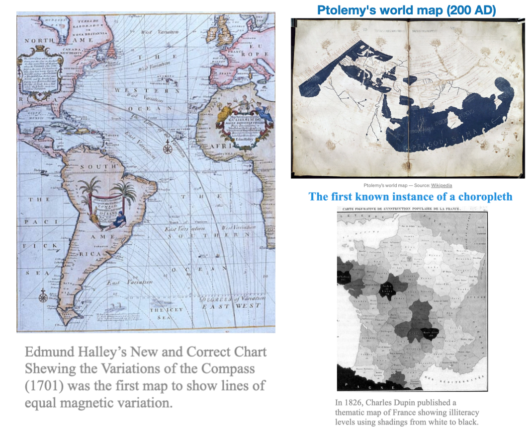
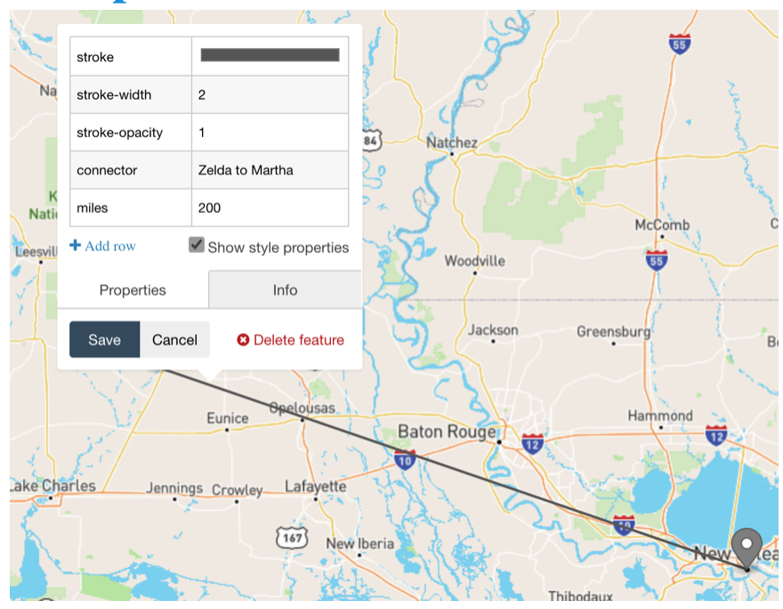
Spatial data has been around for a long time, as we saw in lecture-1, the first data visualizers were map makers
Spatial Data: Overview
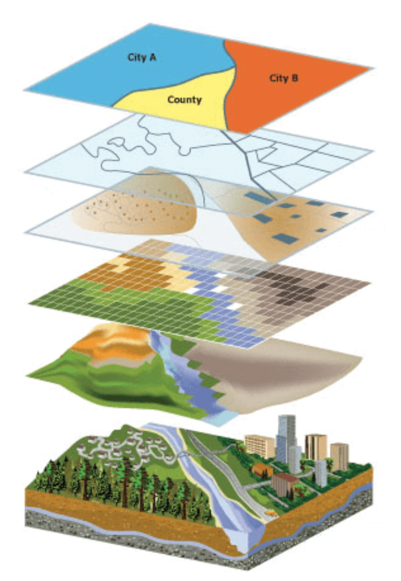
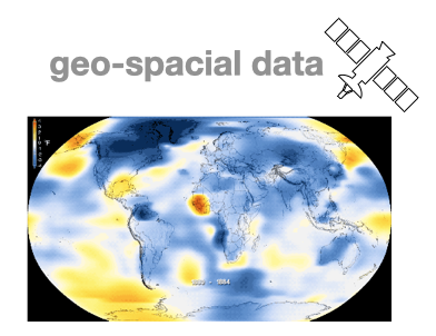
Spatial data, also known as geo-spatial data, is information about a physical object that can be represented by numerical values in a geographic coordinate system.
Spatial data represents:
location, size and shape of an object on planet Earth such as a building, lake, mountain or township
Spatial data may also include attributes that provide more information about the entity that is being represented
Geographic Information Systems (GIS) or other specialized software applications can be used to access, visualize, manipulate and analyze geospatial data
Can be another attribute in a standard tabular dataset
Latitude and longitude are not enough!
Coordinate pairs, are overly simplistic, and lose much of their meaning when treated independently
Typically we are more interested in location AND local attributes
In addition to having point locations, observations may often be associated with spatial lines, areas, or grid cells
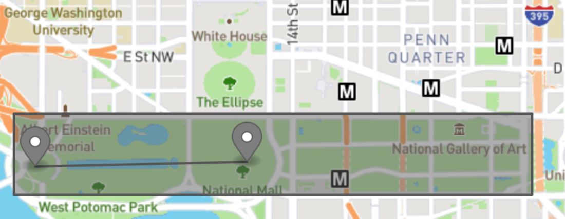
spatial distances between observations are often not well represented by straight-line distances, but by great-circle distances, distances through networks, or by measuring the effort it takes in getting from \(\mathrm{A}\) to \(\mathrm{B}\)
What can we use Spatial analysis for?
Spatial analysis lets us ask, and find answers to, a wide range of questions in six broad categories:
Understanding where things and events are
Measuring sizes, shapes, and distributions of things or measurements
Analyzing relationships and interactions between places
Optimizing locations for facilities, or routes for transportation
Detecting and quantifying patterns and relationships between things or measurements
Making predictions based on existing or theoretical patterns and relationships
For today’s, we focus on visualizing data with a geographical/geo-spatial component.
Geo-spatial: use cases
Using visualizations to understand relationships over space (and also time)
Typically related to data linked with locations or coordinate systems
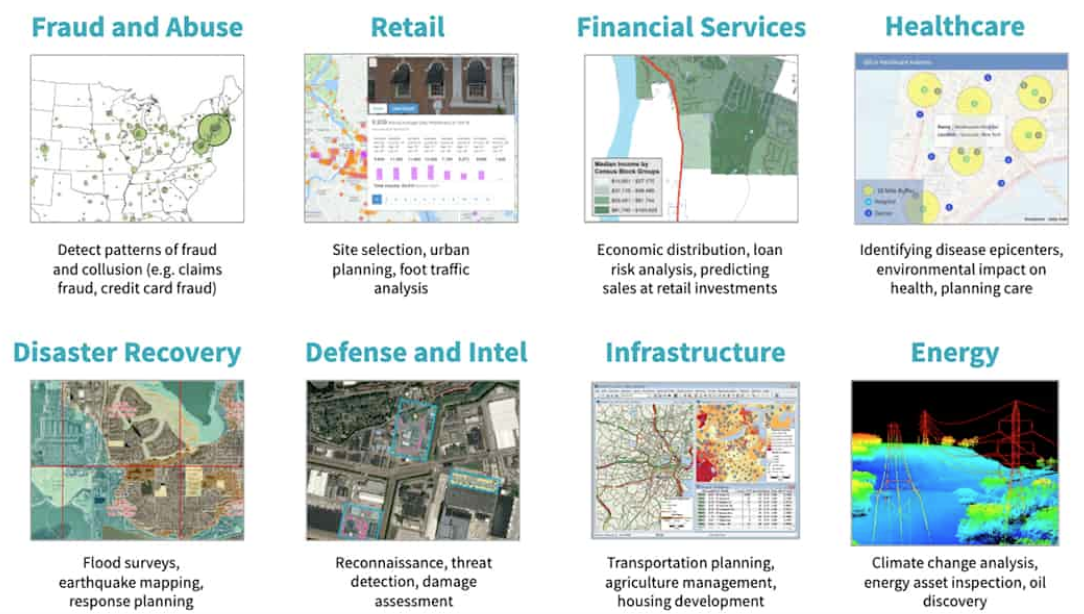
There are many applications
geographic maps, geo-statistics and geographic information systems
medical images (x-rays, MRI, microscopy, pathology)
LIDAR/SONAR/Remote sensing
Epidemiology
Environmental science
meteorology/climatology
urban planning
Applications
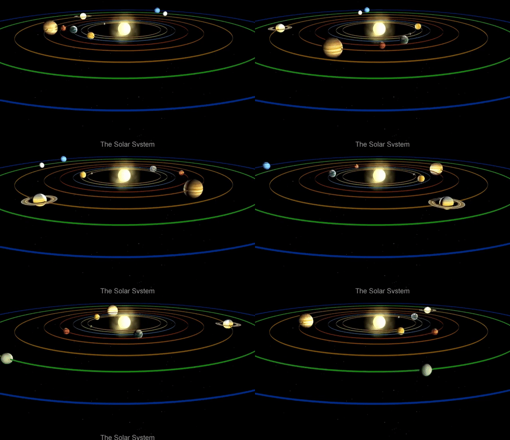
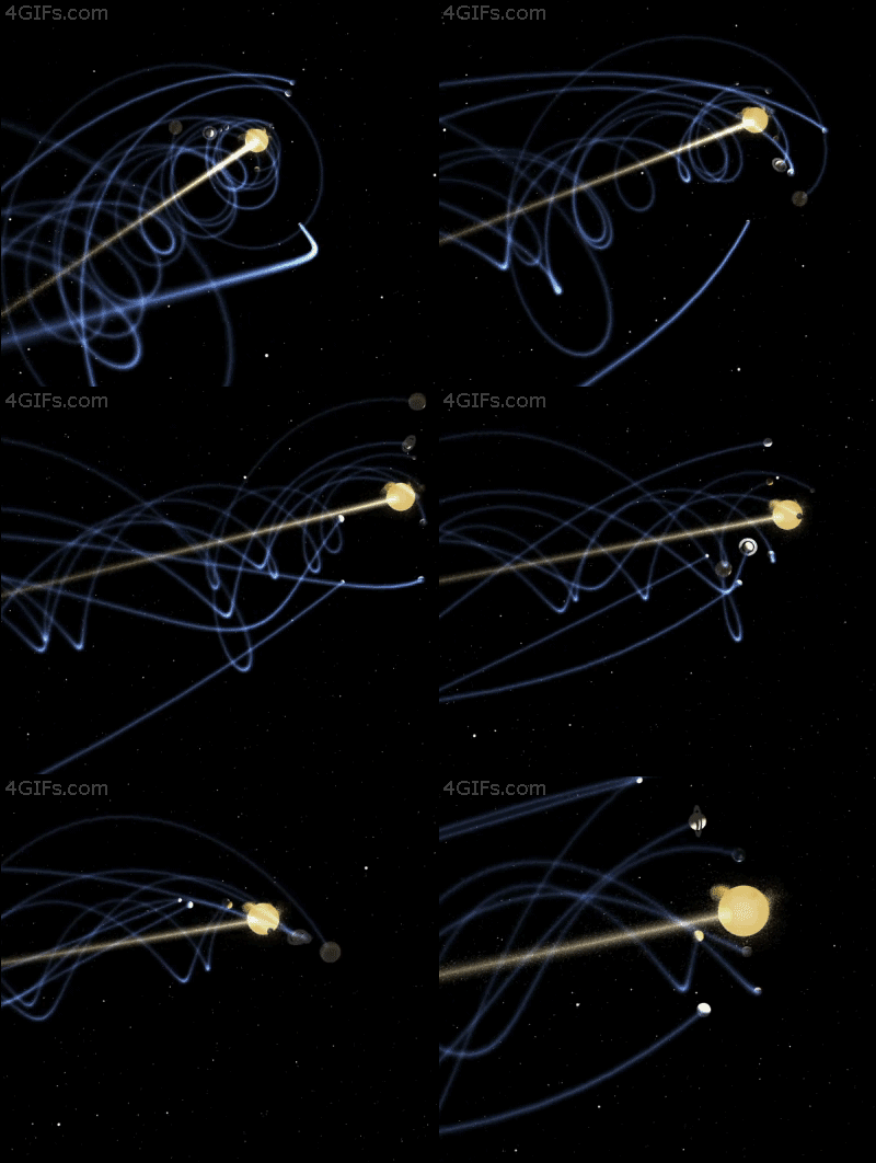
Fun Aside: Physics
Much of physics is inherently “spatial” in nature. In some sense, physics is just a collection of models and laws that describe spatial kinematics of matter in 3D space.
This is a fun gif showing the solar system with a moving sun (as is the case)
Static sun solar system
Moving sun solar system (real case)
Coordinate Reference Systems
CRS
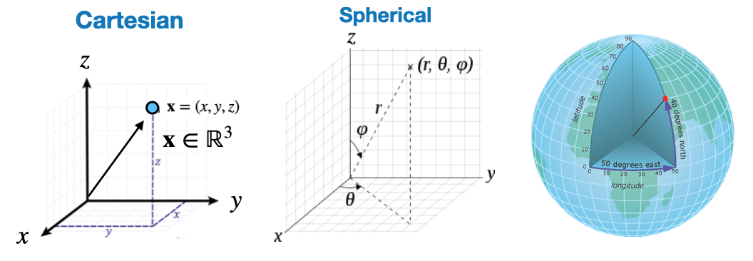
Spherical Coordinate system
We exist in 3D space, which is mathematically represented with coordinate systems
Not surprisingly, spherical coordinates are particularly useful for geo-data
Aside: You can “re-map” coordinates from one space to another with the following: \(\begin{aligned} & r=\sqrt{x^2+y^2+z^2} \,\,\,\,\,\,\,\,\,\,\,\,\,\,\,\,\,\, \theta=\arccos \frac{z}{\sqrt{x^2+y^2+z^2}}=\arccos \frac{z}{r}=\arctan \frac{\sqrt{x^2+y^2}}{z} \\ & \varphi= \begin{cases}\arctan (y / x) & \text { if } x>0 \\ \arctan (y / x)+\pi & \text { if } x<0 \\ \frac{\pi}{2} & \text { else }\end{cases} \end{aligned}\)
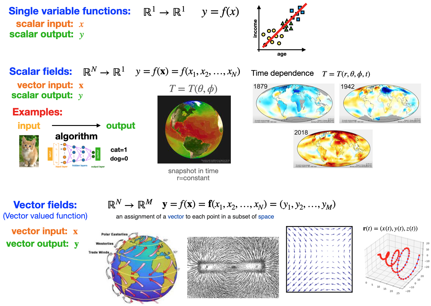
Mathematical relationships
As with other data, Geo-spatial relationships typically fall into the following categories
Overview
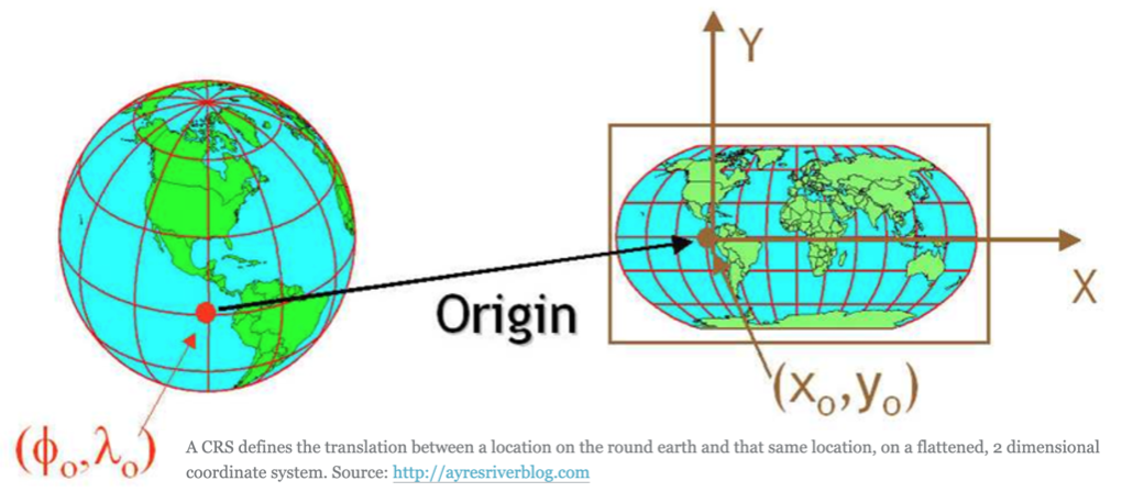
Coordinate reference systems (CRS) are ways to represent the 3D spatial data of earth on a 2-dimensional surface.
A spatial reference system defines a specific map projection, as well as transformations between different spatial reference systems.
CRS: Components
The CRS is a very important aspect of spatial data. For example, a location of (140, 12) on earth is useless without units (meters, KM, miles, degrees) and an origin point.
The coordinate reference system is made up of several key components:
Coordinate system: The X, Y grid upon which your data is overlayed and how you define where a point is located in space.
Horizontal and vertical units: The units to define the grid along the \(x, y\) (and \(z\) ) axis.
Datum: A modeled version of the shape of the Earth which defines the origin used to place the coordinate system in space.
Projection Information: The mathematical equation used to flatten objects that are on a round surface(e.g. the Earth) so you can view them on a flat surface (e.g. your computer screens or a paper map).
Different planar coordinate reference systems are referred to as projections. Examples are ‘Mercator’, ‘UTM’, ‘Robinson’, ‘Lambert’, and ‘Albers’.
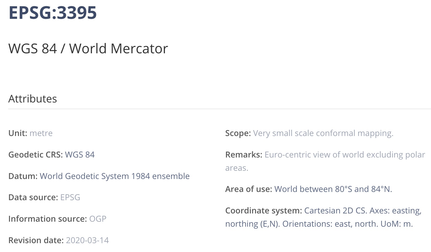
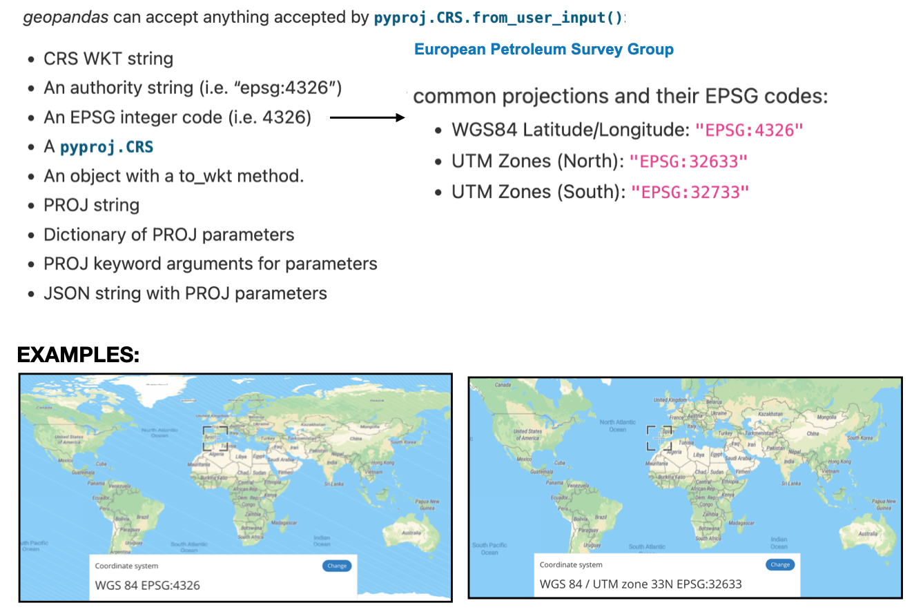
They are typically tagged with EPSG tags to identify them
Note: EPSG=“European Petroleum Survey Group”
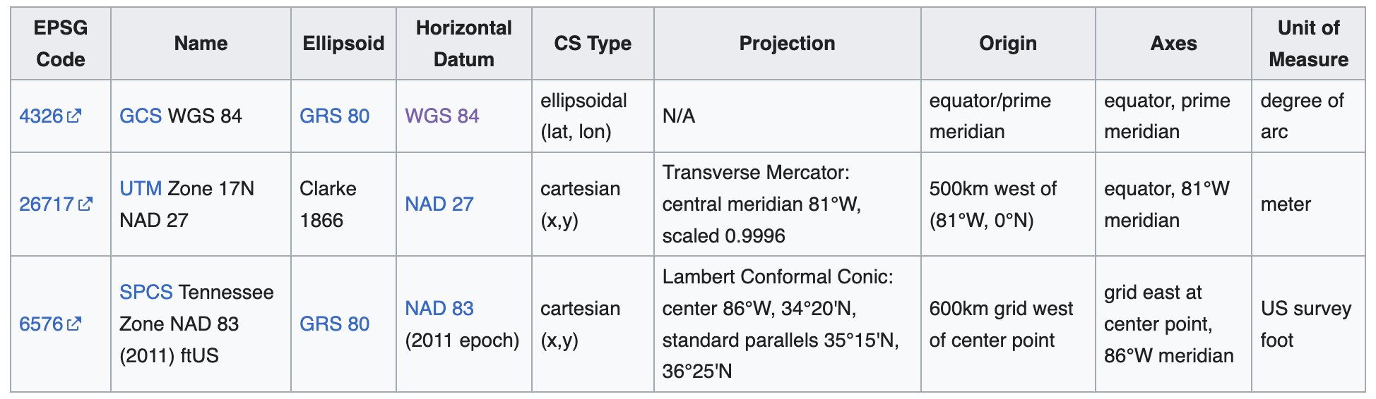
CRS definitions will typically consist of a “stack” of dependent specifications, as exemplified in the following table:
This is a vast field of study, if you specialize in geo-spatial data, then you would need to learn more, however, for now this is enough.
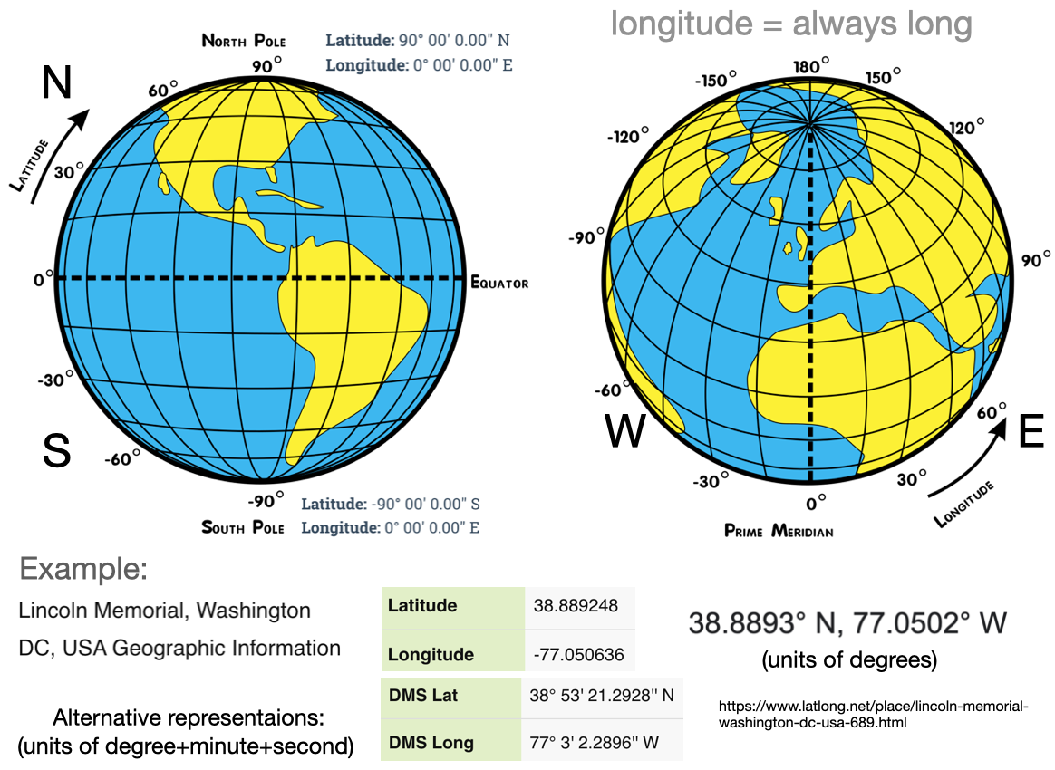
CRS Units: longitude & latitude
Geo-spatial data is often represented in spherical coordinates, with the radius constant
A common choice of units in a CRS is degree’s (longitude & latitude)
Exercise
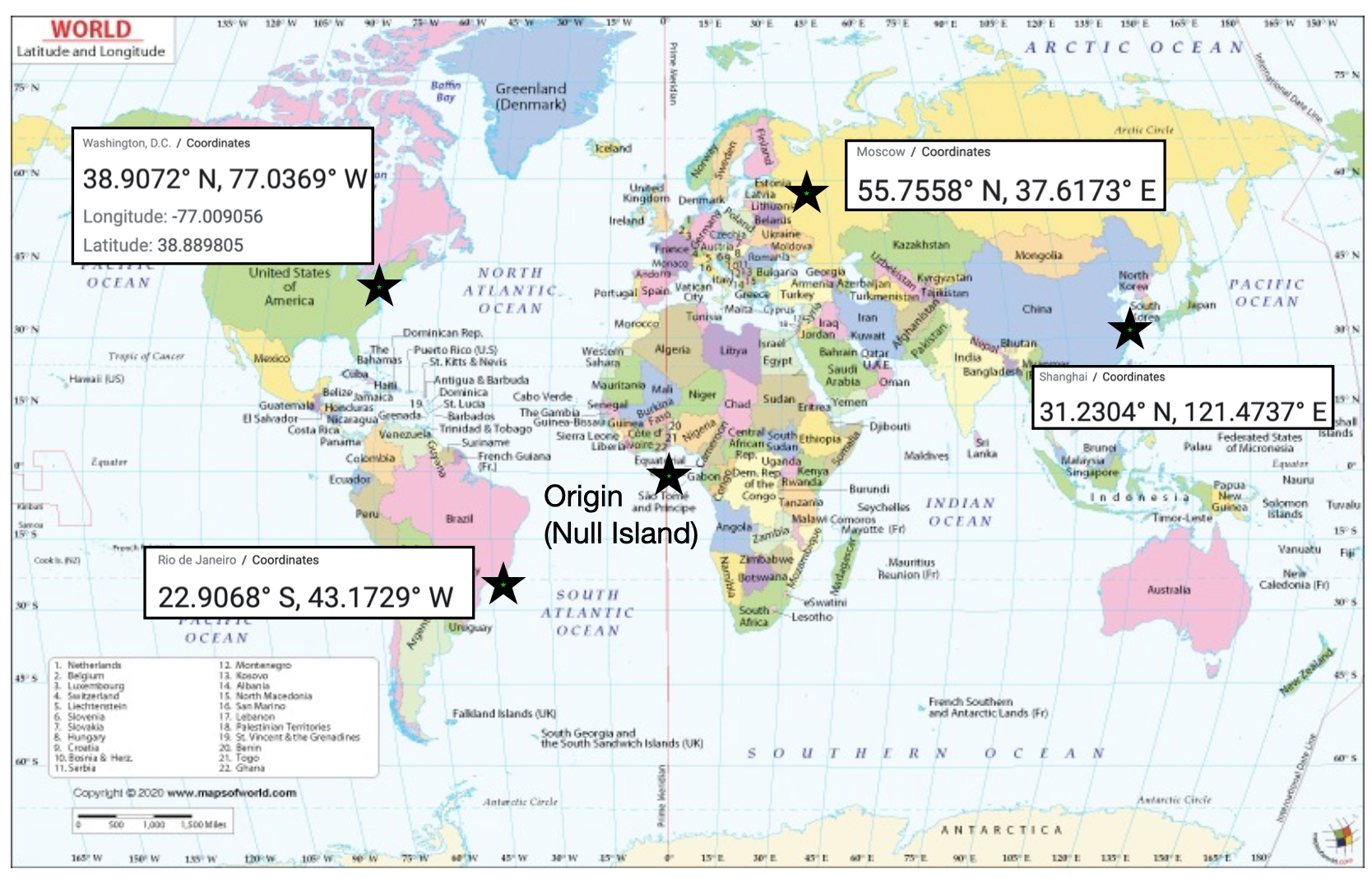
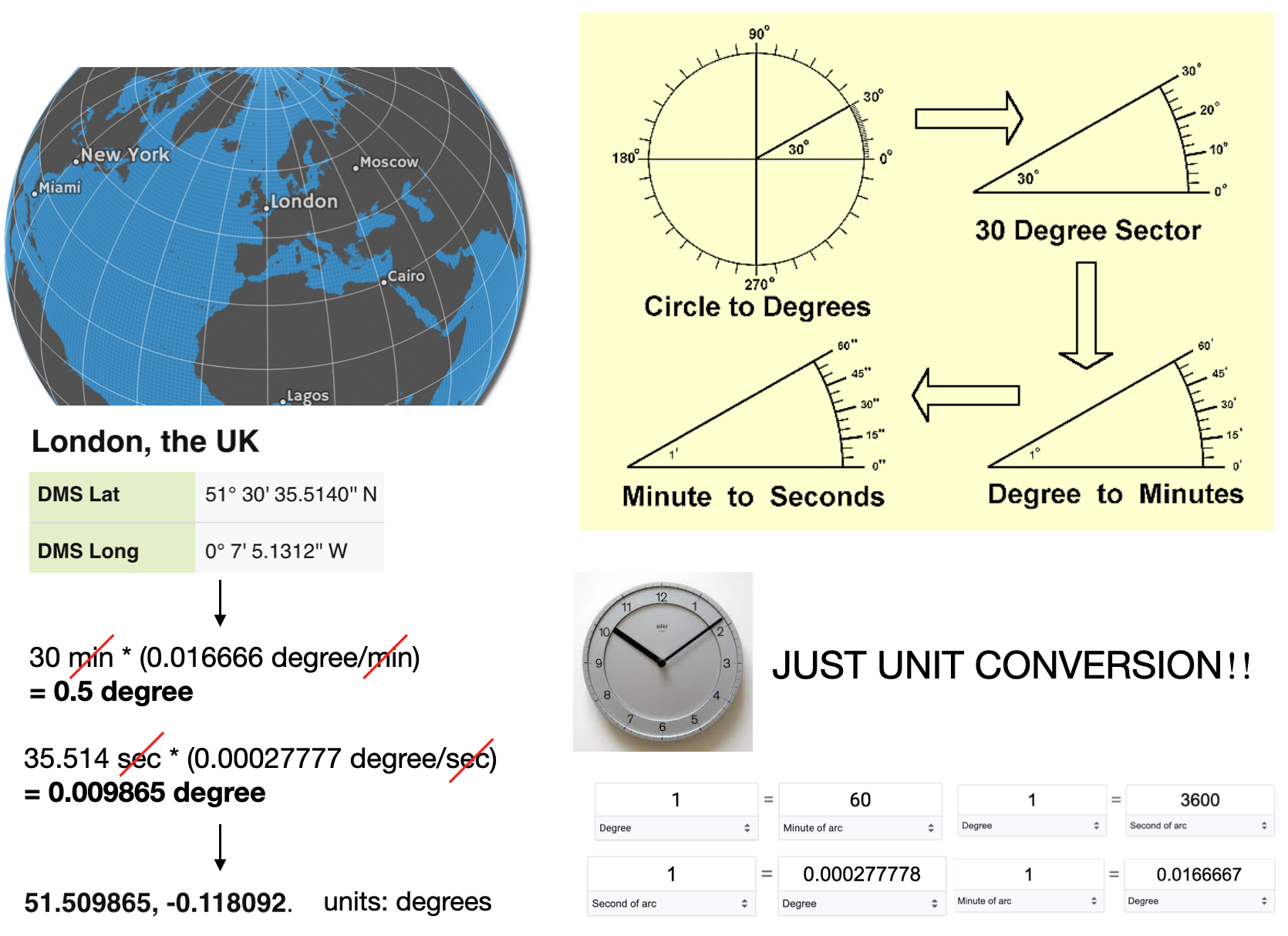
It’s good to be able to estimate locations on earth from longitude & latitude. For example:
CRS Units: Minutes to degrees
London: latitude 51.509865, and longitude -0.118092. (degrees)
CRS Units: Length
Units can also be distance measured from some point (e.g. meters)
When using a CRS, it is good to look it up to determine the units and other details
Attention to detail with units is always important, e.g. measuring area in “degrees squared” doesn’t make a lot of sense.
Sanity check: Earth/Circumference 40.075 million meters
CRS: Map projections
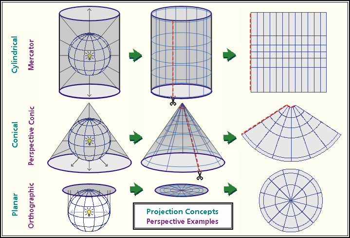
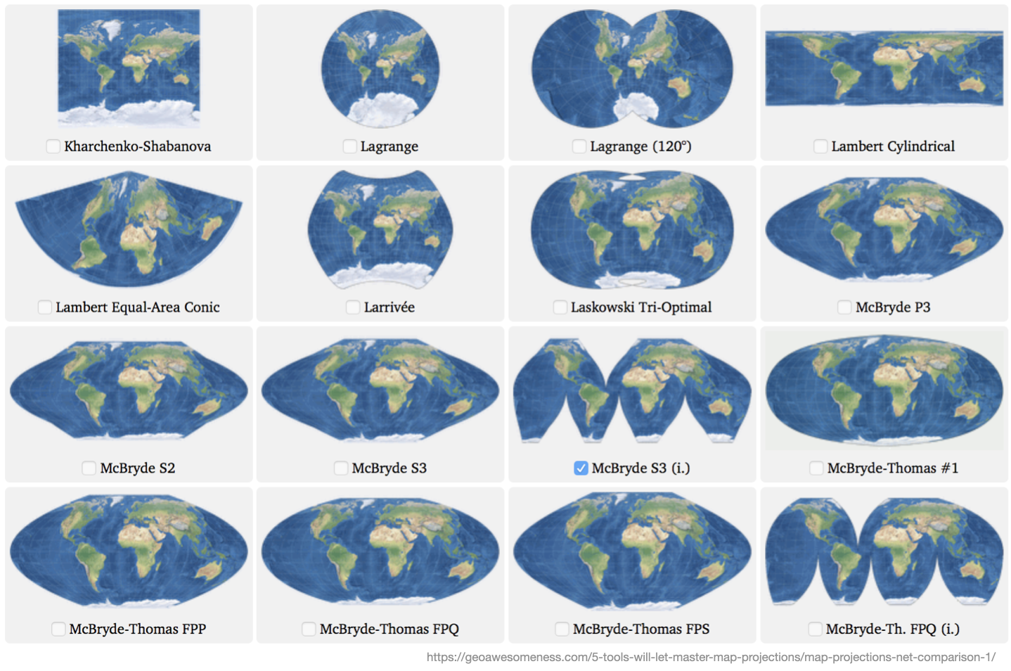
Projection: The mathematics used to flatten objects that are on a round surface
This is a specialized form of dimensionality reduction
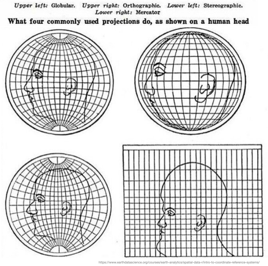
map projection are either “equal area” (the scale of the map is constant) or “conformal” (the shapes of the geographic features are as they are seen on a globe)
Map projects have to be one or the other, they can’t be both
Projection: Examples
CRS: Map projections distortions
Mappings from 3D to 2D always leave artifacts and distortions.
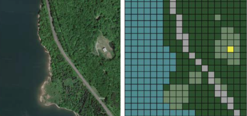
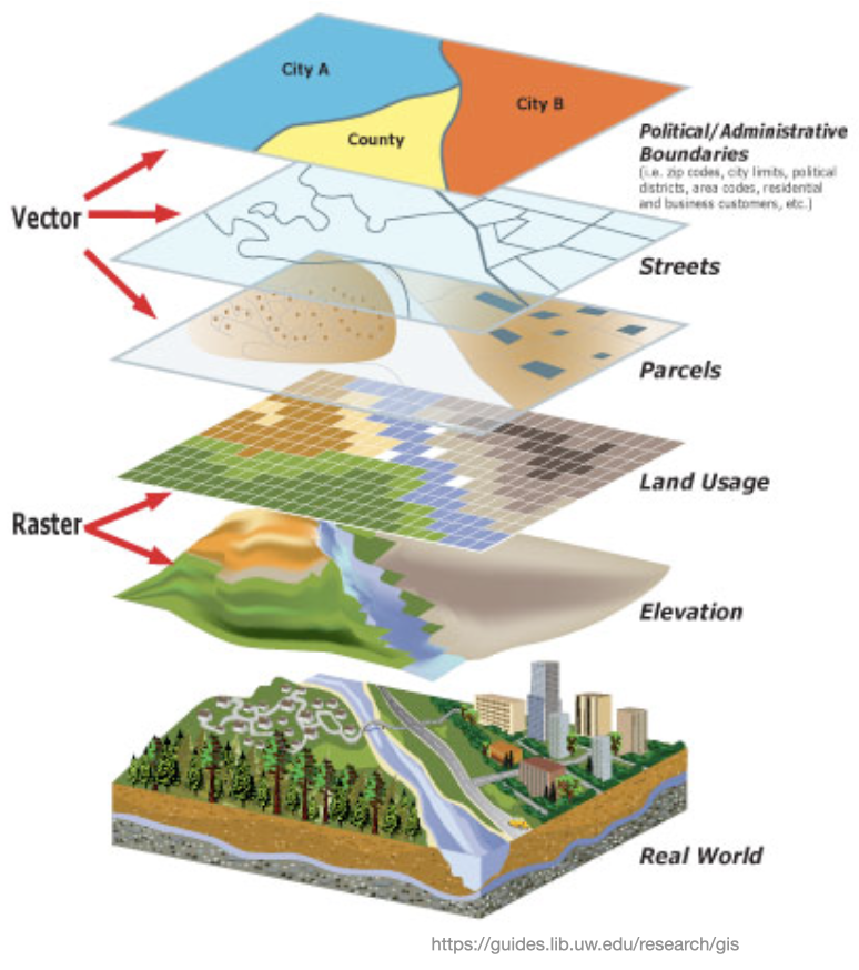
We’ve seen raster & vector graphics before, but, the concepts are also important for geo-data
Raster GIS Formats Raster data is made of pixels (grid cells) with associated values (continuous) or class (discrete). They are usually regularly spaced squares but don’t have to be.
Vector GIS Formats: Not made up of grids of pixels. Instead, vector graphics are comprised of vertices and paths (points, lines, and polygons).
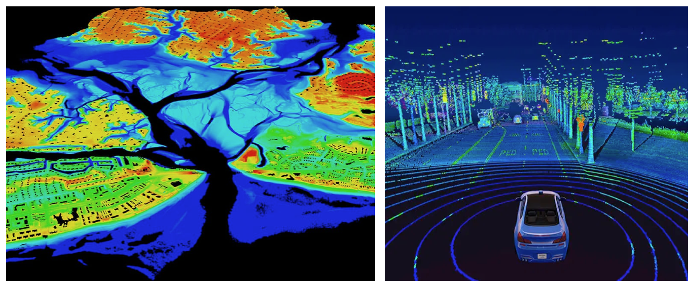
In addition to raster and vector data, there is also LiDAR data (also known as point clouds) and 3D data. LiDAR data is data that is collected via satellites, drones, or other aerial devices. 3D data is data that extends the typical latitude and longitude 2-D coordinates and incorporates elevation and or depth into the data. While complex, this data is rich with information and can be used to solve a variety of problems pertaining to the Earth’s surface.
Geo-spatial file-formats
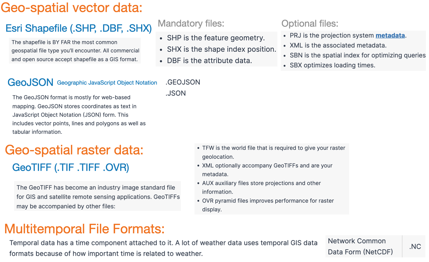
There are MANY formats for storing Geo-spatial data, here are some popular choices.
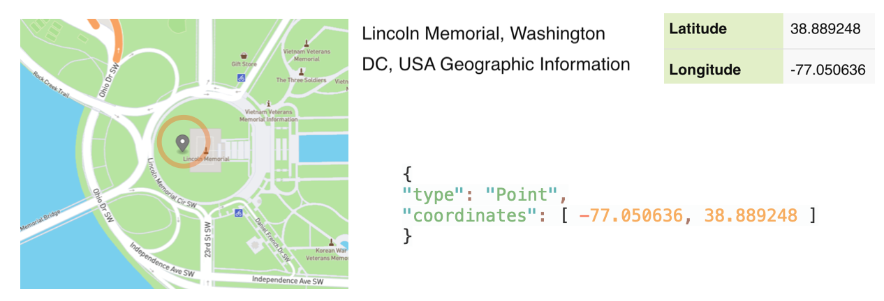
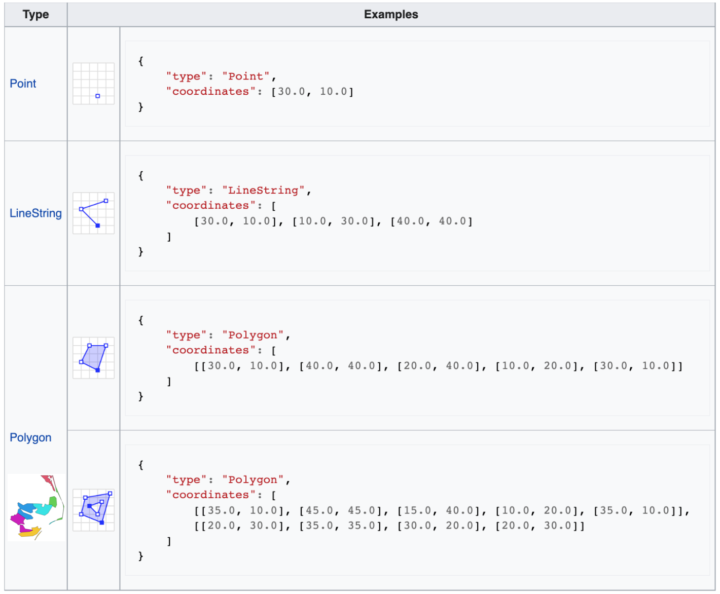
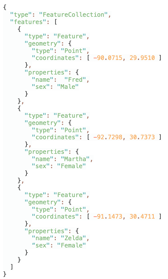
GeoJSON is an open standard format designed for representing simple geographical locations, along with their non-spatial attributes.
GeoJSON consists of the following parts:
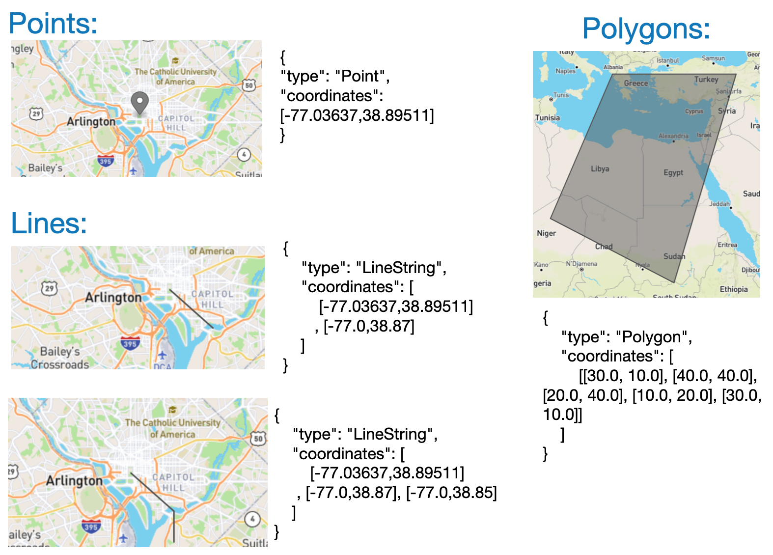
Geometry object: point, line, or polygon composing location information. Points are [x, y] or [x, y, z]. They may be [longitude, latitude ] or [eastings, northings]. Elevation is an optional third number.
Good resource: https://developer.here.com/blog/an-introduction-to-geojson
Geo-Json: Geometry primitives
Geo-Json: Geometry examples
Here are additional examples of geographic information stored in the Geo-Json format
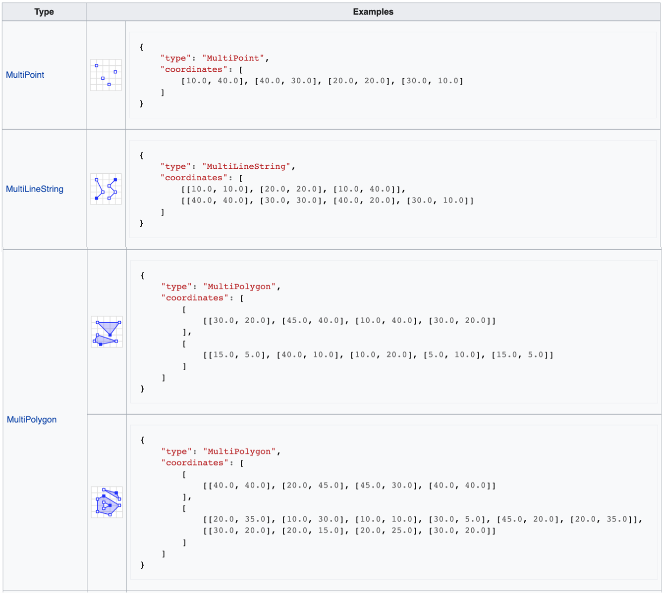
Geo-Json: Multipart geometries
We can also store collections of geometric primitives in groups
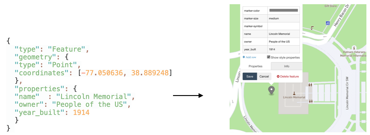
Geo-Json: components
Feature object: This is the geometry object & the associated meta data. This can be anything associated with that location or region
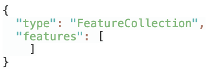
FeatureCollection: Basically just a list of feature objects. This can be used to collect different categories of features
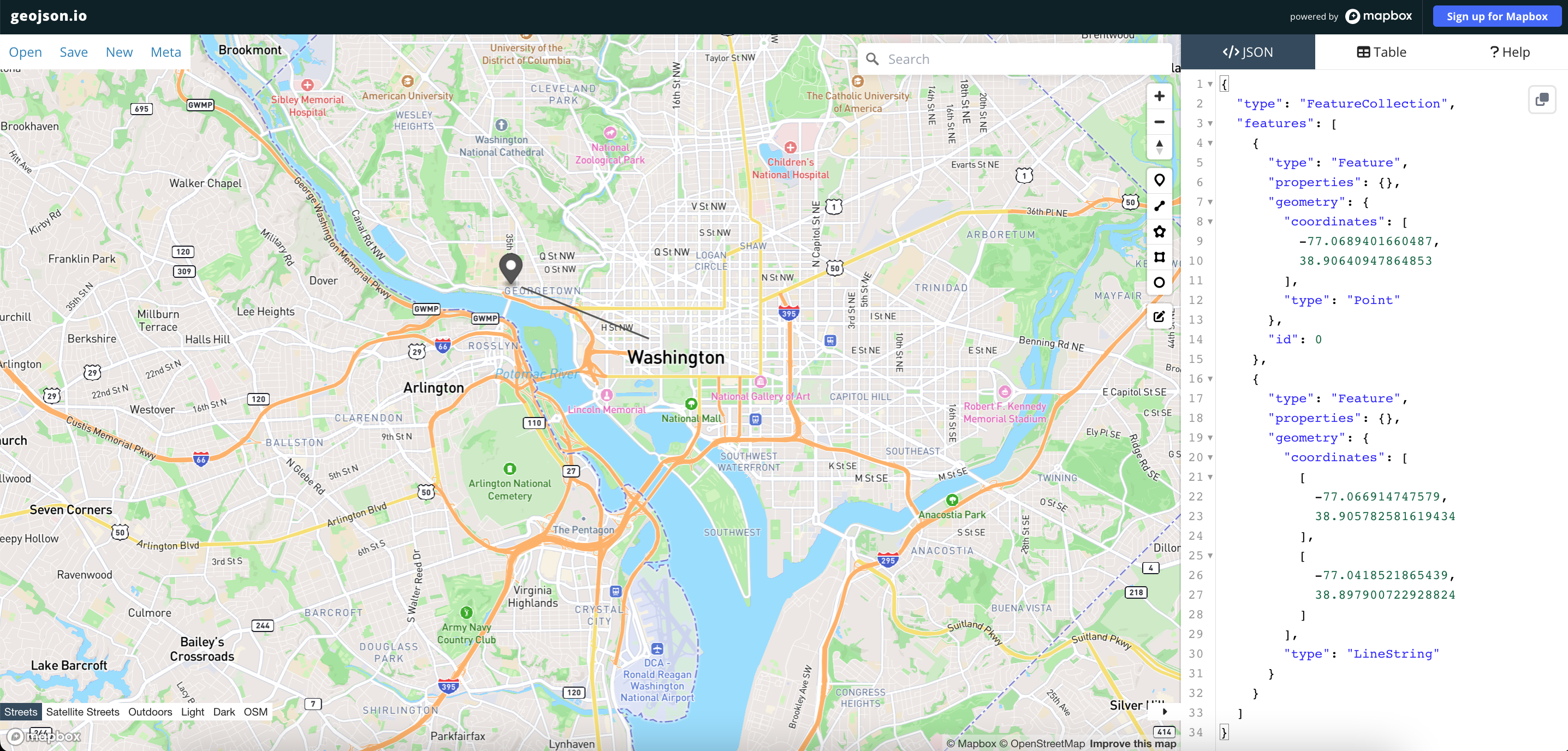
Optional: Demonstration
The following lets you build up a geo-Json file from scratch: run demo (optional)
Shape files
The shape-file is an alternative to GeoJSON, it is BY FAR the most common geospatial file, since it is used by GIS.
The term “shapefile” is quite common, but the format consists of a collection of files with a common filename prefix, stored in the same directory.
Mandatory files
shp - Main file: a direct access, variable-record-length file in which each record describes a shape with a list of its vertices.
shx - Index file: each record contains the offset of the corresponding main file record from the beginning of the main file. The index file (.shx) contains a 100-byte header followed by 8-byte, fixed-length records.
dbf - dBASE Table file: a constrained form of DBF that contains feature attributes with one record per feature. The one-toone relationship between geometry and attributes is based on record number. Attribute records in the dBASE file must be in the same order as records in the main file.
One downside, the files are stored as binary objects and are not human readable
Interactive mapping packages
Java-script libraries
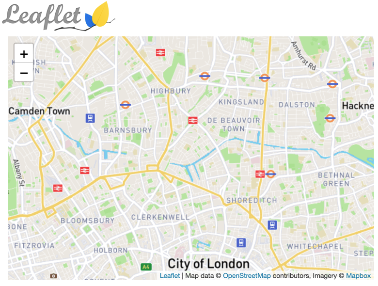
Leaflet.js
Popular open-source JS library for embedding mobile-friendly interactive maps.
Very light-weight, at around 38 KB of JS, it has all the mapping features most developers ever need.
Leaflet.js provides the mapping tools, the data comes from map data-bases.
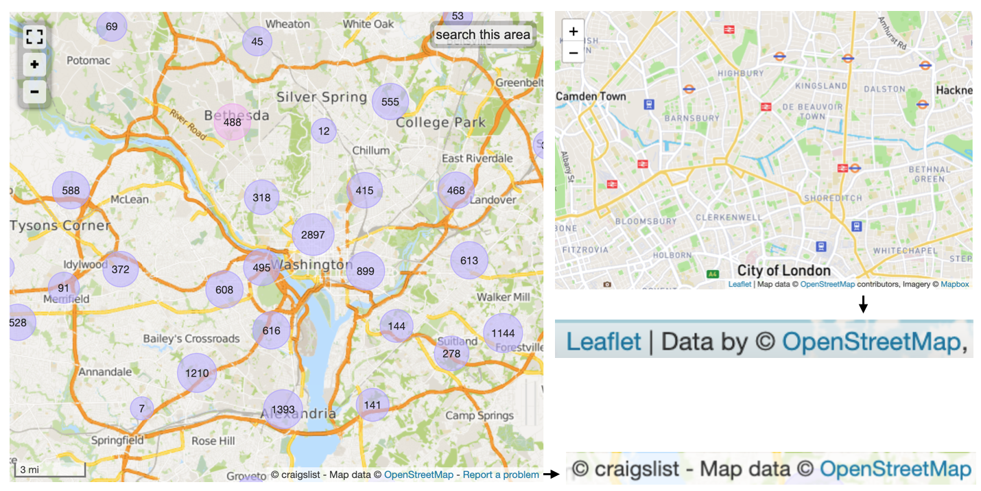
Map database: OpenStreetMap
OpenStreetMap (OSM) is a collaborative project to create a free editable geographic database of the world by the OpenStreetMap Foundation (OSMF).
It is licensed under the Open Data Commons Open Database License (ODbL)
OpenStreetMap.org provides a map interface based on the Leaflet JavaScript library
Google also has it’s own map data-base as an alternative to OSM
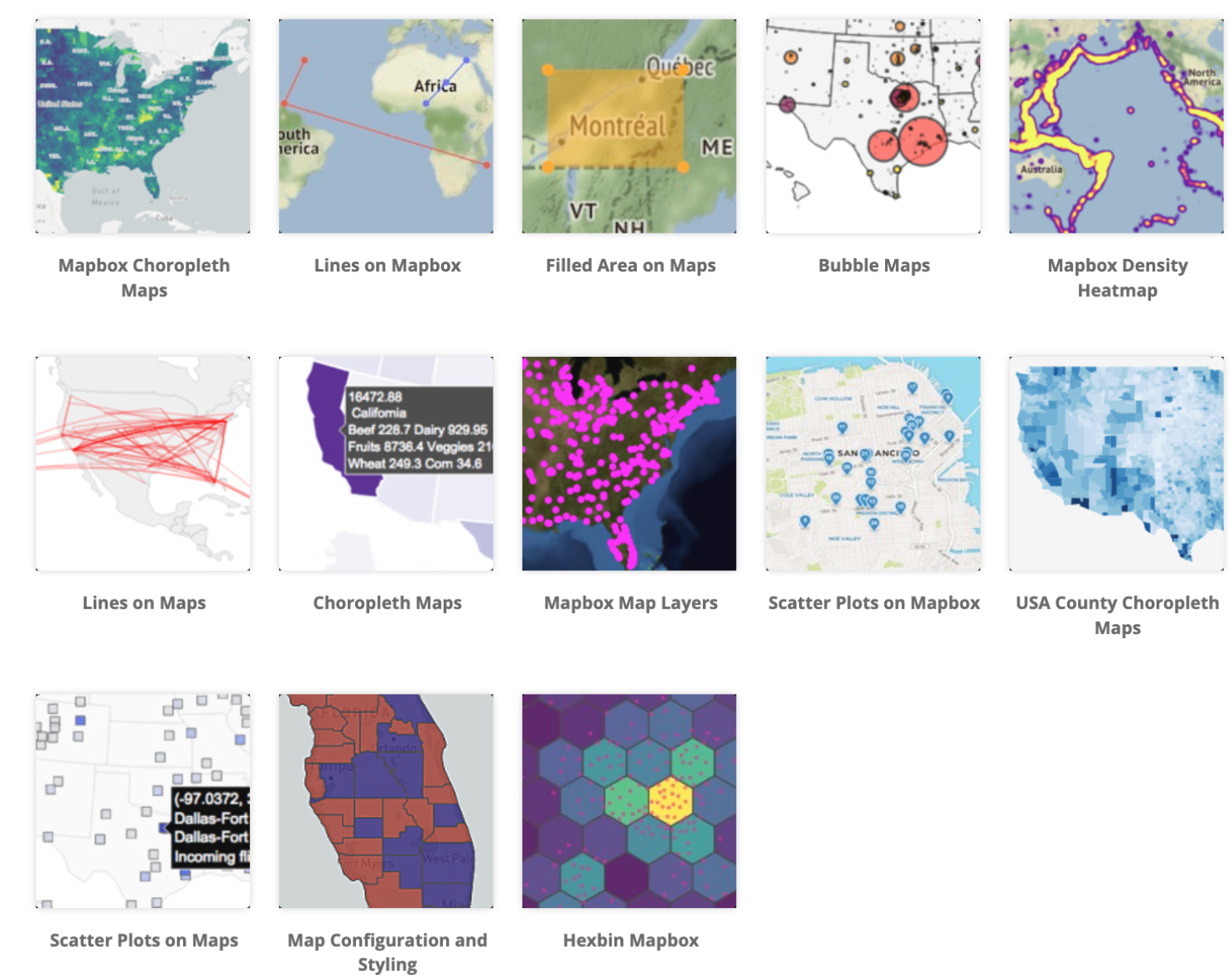
Leaflet.js alternative \(\rightarrow\) Mapbox GL JS
Mapbox GL JS is a client-side JavaScript library for building web maps and web applications with Mapbox’s modern mapping technology.
You can use Mapbox GL JS to display Mapbox maps in a web browser or client, add user interactivity, and customize the map experience in your application.
Similar to OpenStreetMap, the Mapbox also provides a popular geographic database
Source: [click here for more)(https://docs.mapbox.com/mapbox-gl-js/guides/)
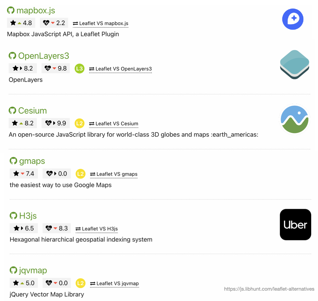
Leaflet.js Alternatives
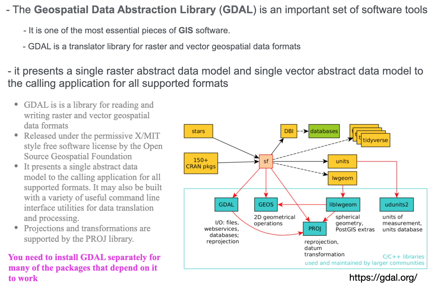
GDAL
Geo-spatial visualization
Introduction to geo-spatial visualization in Python.
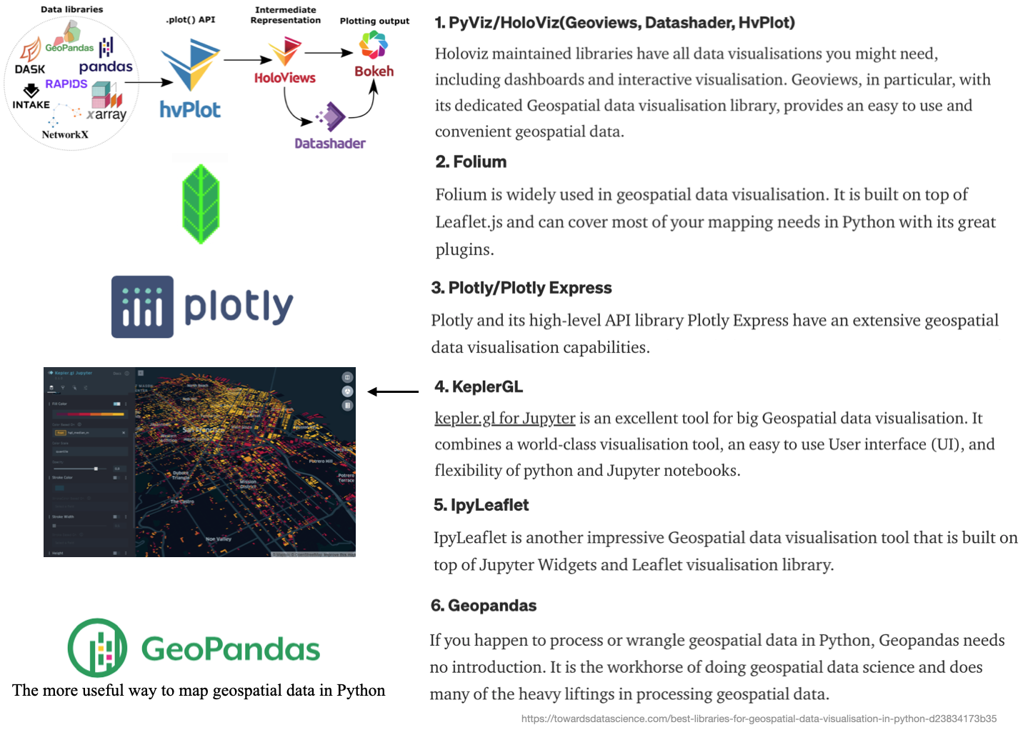
Python: Common Geo-spatial packages
Note: This is not in any particular order
Geo-pandas
The most useful way to map geospatial data in Python is geopandas.
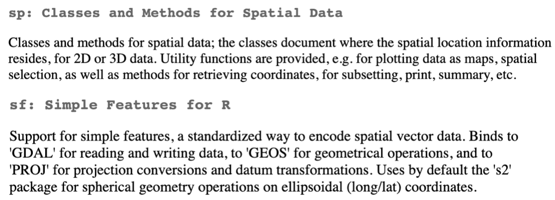
This works very similarly to the sf package in \(\mathrm{R}\)
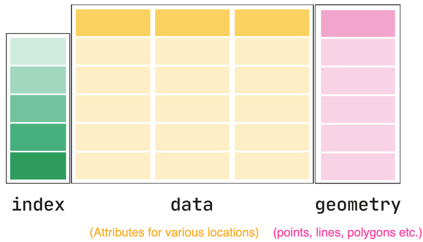
All the data in one pandas. DataFrame-like object
One column for the simple features geometry specification (called geometry)
Other columns for data about each geometry, that you can then represent within a map
There are some basic plotting functions with Geo-pandas, built on MPL
Note: We cover GeoPandas more in the lab, so we only show the basics here
The core data structure in GeoPandas is the geopandas.GeoDataFrame
It is a modified data-frame to store geometry and perform spatial operations.
geopandas.GeoSeries, a subclass of pandas.Series, handles the geometries
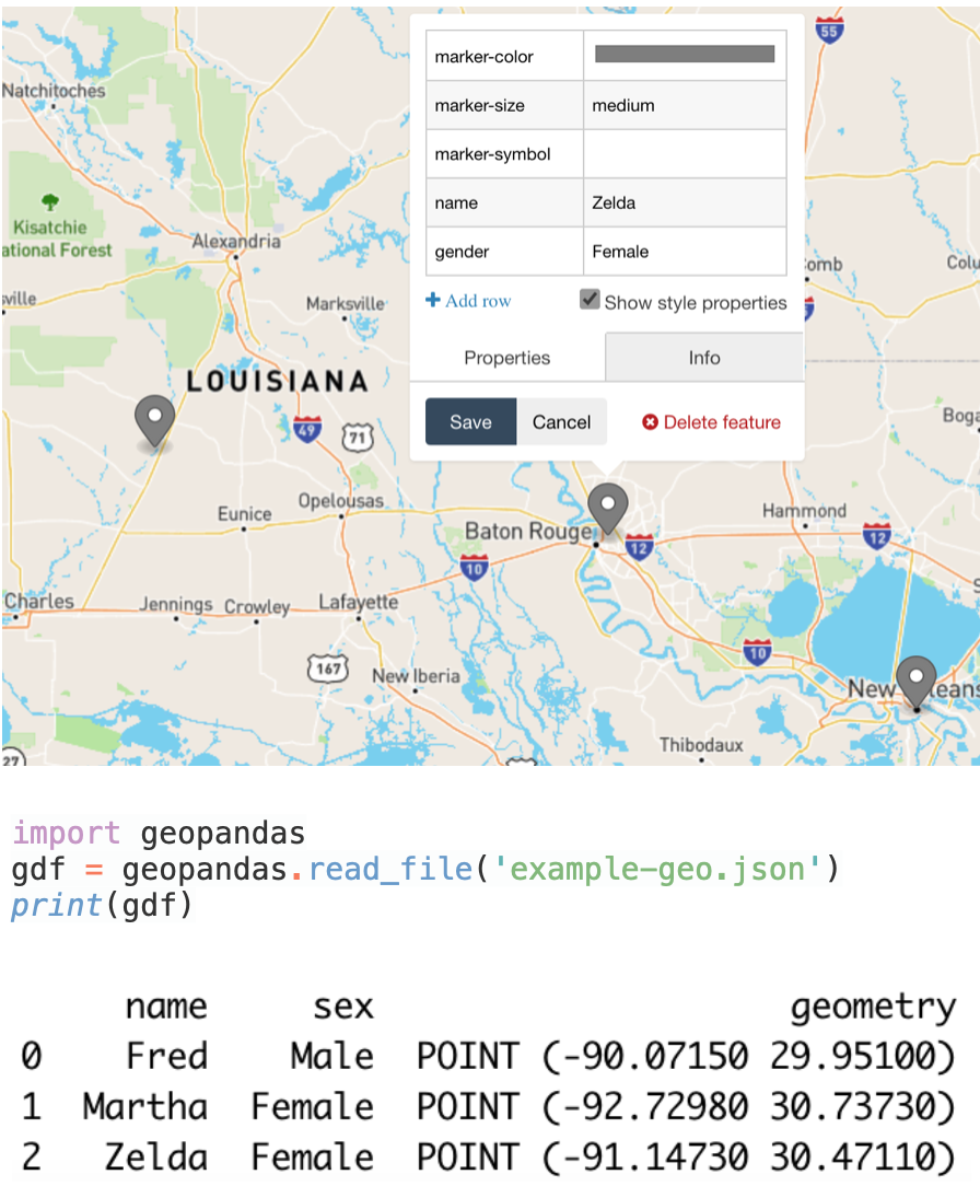
Geo-pandas: Data Frames example-1
Input data: GeoJson
Resultant data frame
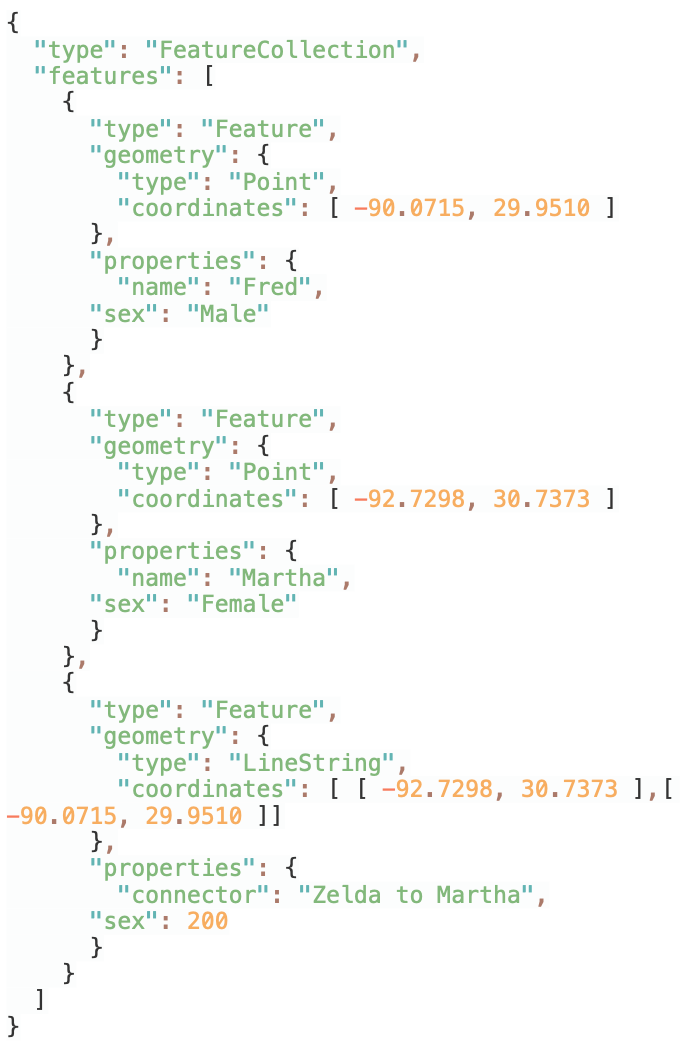
Geo-pandas: Data Frames example-2
Input data: GeoJson
Map
Data frame
Geopandas: CRS
GeoSeries.crs attribute, stores information about the projection and CRS
Code example: Python
Code
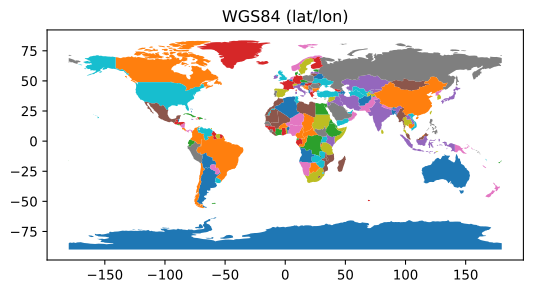
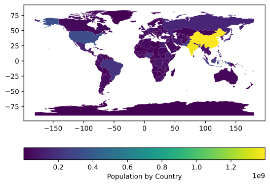
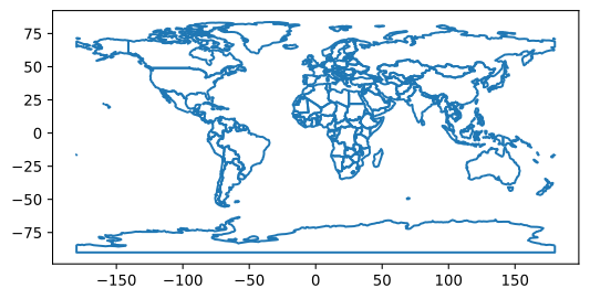
import geopandasimport matplotlib.pyplot as plt# GET DATAPATH =geopandas.datasets.get_path("naturalearth_lowres")# READgdf =geopandas.read_file(PATH)# PLOT: W/ MATPLOTLIBfig, ax =plt.subplots()ax =gdf.plot("name", legend=False, ax=ax)ax.set_title("WGS84 (lat/lon)")plt.show()# plt.clf()
CRS: Units and Measures
Again the CRS units are very important, as they effect anything you measure
Code
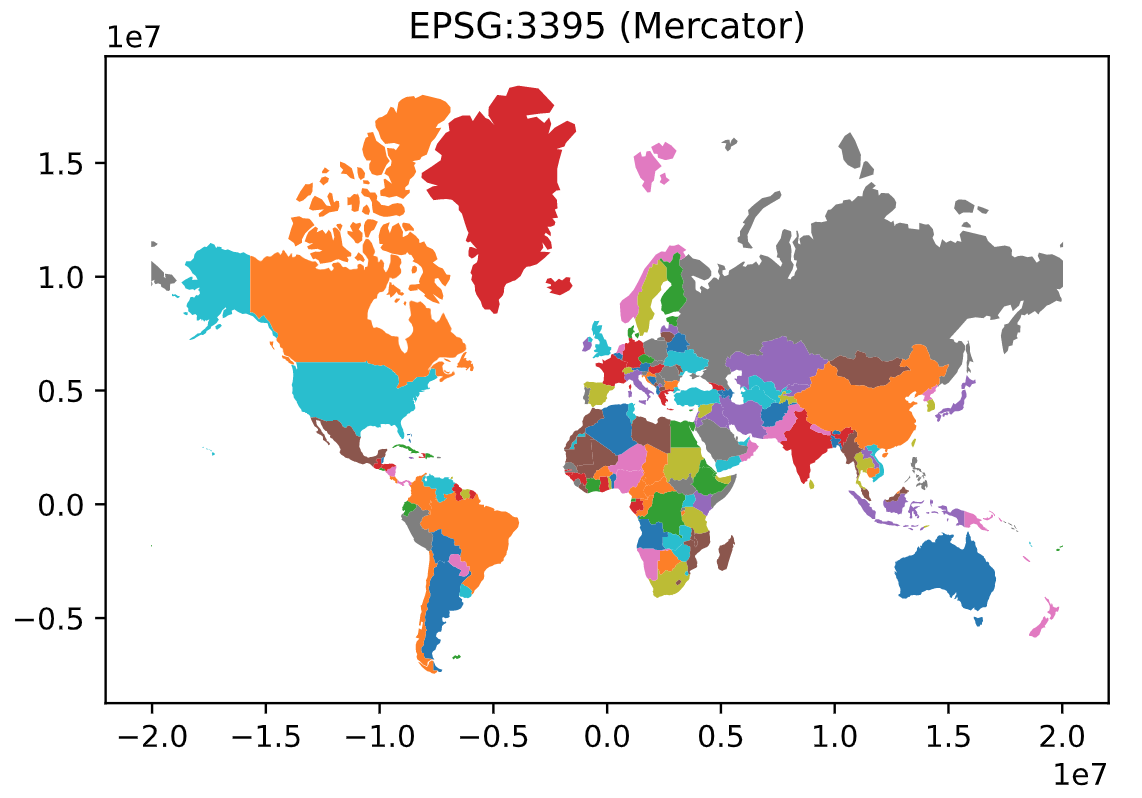
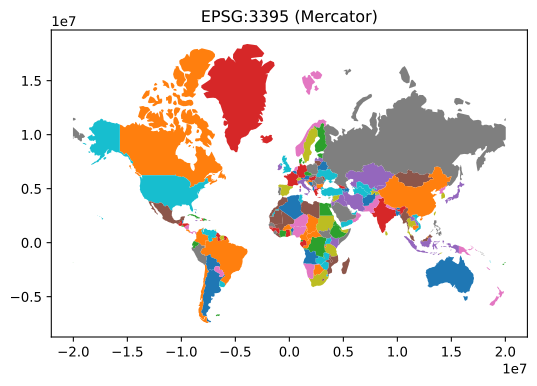
import geopandas #GET DATAPATH =geopandas.datasets.get_path("naturalearth_lowres")# READgdf =geopandas.read_file(PATH)gdf =gdf.to_crs("EPSG:3395") #CHANGE CRS TO 3395#MEASURE THE AREA OF EACH POLYGON: access the GeoDataFrame.areagdf["area"]=gdf.area; #print(gdf)#SANITY CHECK GOOGLE: Tanzania/Area --> 364,900 mi^2 9.450867e+11 m^2print(gdf.loc[gdf['name'] =="Tanzania"])#NEED TO BE CAREFUL WITH MULTI-POLYGON COUNTRIES (AREAS INCORRECT)
      pop_est continent      name iso_a3  gdp_md_est  \
1  58005463.0    Africa  Tanzania    TZA       63177

                                            geometry          area
1  POLYGON ((3774143.866 -105050.440, 3792946.708...  9.459693e+11
ALWAYS check to make sure your numbers make sense and are meaningful!
import pandas as pdimport matplotlib.pyplot as pltimport geopandas as gpworld =gp.read_file(gp.datasets.get_path('naturalearth_lowres'))print(world.head())print(world.columns)
       pop_est      continent                      name iso_a3  gdp_md_est  \
0     889953.0        Oceania                      Fiji    FJI        5496
1   58005463.0         Africa                  Tanzania    TZA       63177
2     603253.0         Africa                 W. Sahara    ESH         907
3   37589262.0  North America                    Canada    CAN     1736425
4  328239523.0  North America  United States of America    USA    21433226

                                            geometry
0  MULTIPOLYGON (((180.00000 -16.06713, 180.00000...
1  POLYGON ((33.90371 -0.95000, 34.07262 -1.05982...
2  POLYGON ((-8.66559 27.65643, -8.66512 27.58948...
3  MULTIPOLYGON (((-122.84000 49.00000, -122.9742...
4  MULTIPOLYGON (((-122.84000 49.00000, -120.0000...
Index(['pop_est', 'continent', 'name', 'iso_a3', 'gdp_md_est', 'geometry'], dtype='object')
Folium is a Python library which wraps around leaflet.js to create Leaflet maps.
Due to the interactivity, Folium is useful for dashboard creation, e.g. w/ Streamlit .
Example: initialize a map:
Code
import foliumfrom IPython.display import display# INITIALIZE MAP m =folium.Map(location=[38.907852, -77.072807])# SAVEfile_name="img/map-0.html"m.save(file_name)# RE-LOAD AS AN IFRAMEfrom IPython.display import IFrameIFrame(src=file_name, width=800, height=400)
Folium layers: Markers and circles
Markers can be added to folium maps with folium.Marker and add_to functions. After creating you map you will ble able to add the marker, specifying the desired location, as in the example below.
Code
# https://python-charts.com/spatial/interactive-maps-folium/import foliumm =folium.Map(location = [34.06, -118.25], zoom_start =8)# Add a marker to the mapfolium.Marker(location = [34.06, -118.25]).add_to(m)# Circle with a radius of 50kmfolium.Circle(location = [33.56, -116.85],radius =50000,color ="black",fill = True,fill_color ="blue").add_to(m)# SAVEfile_name="img/map-1.html"m.save(file_name)# RE-LOAD AS AN IFRAMEfrom IPython.display import IFrameIFrame(src=file_name, width=800, height=400)
Folium layers: Polygons from GeoJSON
It is possible to add polygons to the folium maps with the GeoJson function. You just need to pass the geojson file to data, set a name to the layer with name and add optional styling with style_function.
In case you have too many markers you can cluster them with MarkerCluster depending on the zoom level. You can also click over the clusters to zoom over them.
Code
# https://python-charts.com/spatial/interactive-maps-folium/import foliumfrom folium import pluginsimport numpy as np# RANDOMLY SAMPLE LONGITUDES AND LATITUDESdata =np.array([np.random.uniform(low =25, high =50, size =100),np.random.uniform(low =-125, high =-70, size =100)]).T# INITIALIZE MAPm =folium.Map([40, -100], zoom_start =3)# ADD POINTS plugins.MarkerCluster(data).add_to(m)# SAVEfile_name="img/map-5.html"m.save(file_name)# RE-LOAD AS AN IFRAMEfrom IPython.display import IFrameIFrame(src=file_name, width=800, height=400)
import pandas as pdimport plotly.express as px# GET DATAdf =pd.read_csv("https://raw.githubusercontent.com/plotly/datasets/master/earthquakes-23k.csv")# LOOK AT DATA STRUCTUREprint(df.head(1))# GENERATE PLOTfig =px.density_mapbox( df,lat="Latitude",lon="Longitude",z="Magnitude",radius=10,center=dict(lat=0, lon=180),zoom=0,mapbox_style="stamen-terrain",)# fig.show()# SAVEfile_name="img/plotly-3.html"fig.write_html(file_name)# RE-LOAD AS AN IFRAMEfrom IPython.display import IFrameIFrame(src=file_name, width=1000, height=500)
         Date  Latitude  Longitude  Magnitude
0  01/02/1965    19.246    145.616        6.0
Plotly: Dot map
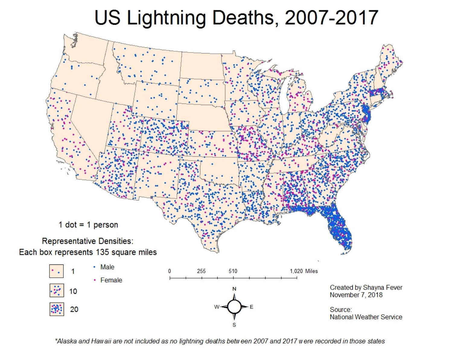
A dot map (also called dot distribution map or dot density map) uses a dot to indicate the presence of a variable.
Dot maps are essentially scatterplots on a map and are used to show spatial patterns.
Dots are often used in graphs, charts, and maps to accurately locate individual observations and phenomena, but that’s not the case here. If you read a dot density map that way, it’ll look like there were fatalities everywhere in Florida, and that lightning strikes become much less deadly as soon as you cross the border with Georgia or Alabama.
In a dot density map, though, each dot represents one observation, but dots aren’t located where those observations were made; instead, dots are distributed to maximize coverage and, if the placement algorithm is well designed and manually tweaked, it’ll avoid absurd placement —such as dots over lakes, rivers, or unpopulated regions.
Plotly: Bubble maps
Bubble maps summarize your data by creating different sized circles that represent the value of the information in each geographic area.
The larger the bubble, the higher the value of your data in that area.
Code
import plotly.graph_objects as goimport pandas as pddf =pd.read_csv('https://raw.githubusercontent.com/plotly/datasets/master/2014_us_cities.csv')df.head()df['text'] = df['name'] +'<br>Population '+ (df['pop']/1e6).astype(str)+' million'limits = [(0,2),(3,10),(11,20),(21,50),(50,3000)]colors = ["royalblue","crimson","lightseagreen","orange","lightgrey"]cities = []scale =5000fig =go.Figure()for i inrange(len(limits)): lim = limits[i] df_sub = df[lim[0]:lim[1]]fig.add_trace(go.Scattergeo(locationmode ='USA-states',lon = df_sub['lon'],lat = df_sub['lat'],text = df_sub['text'],marker =dict(size = df_sub['pop']/scale,color = colors[i],line_color='rgb(40,40,40)',line_width=0.5,sizemode ='area' ),name ='{0} - {1}'.format(lim[0],lim[1])))fig.update_layout(title_text ='2014 US city populations<br>(Click legend to toggle traces)',showlegend = True,geo =dict(scope ='usa',landcolor ='rgb(217, 217, 217)', ) )# SAVEfile_name="img/plotly-5.html"fig.write_html(file_name)# RE-LOAD AS AN IFRAMEfrom IPython.display import IFrameIFrame(src=file_name, width=1000, height=450)
Plotly: Hex map
A hex map geographic representation consisting of hexagonal tiles arranged in a honeycomb pattern, commonly used in strategy games and mapping applications.
To use mapbox-styles requiring a mapbox token, set the token with plotly.express. px.set_mapbox_access_token(open(".mapbox_token").read())
Alternatively you can use fig.update_layout(mapbox_style="open-street-map") without a token
Code
import pandas as pdimport plotly.figure_factory as ffdf =px.data.carshare()import plotly.express as pxfig =ff.create_hexbin_mapbox(data_frame=df, lat="centroid_lat", lon="centroid_lon",nx_hexagon=10, opacity=0.9, labels={"color":"Point Count"},)fig.update_layout(margin=dict(b=0, t=0, l=0, r=0))fig.update_layout(mapbox_style="open-street-map") # fig.update_layout(margin={"r":0,"t":0,"l":0,"b":0})# SAVEfile_name="img/plotly-6.html"fig.write_html(file_name)# RE-LOAD AS AN IFRAMEfrom IPython.display import IFrameIFrame(src=file_name, width=1000, height=300)
Possible geo-visualization issues
Some immediate gotcha’s when working with geo-spatial data and trying to create visualizations
Layers won’t match up
Points will not show up on the right location on the grid
Distances won’t be correct
Circles turn to ellipses for no apparent reason
Geographic elements look weird
Geo-spatial visualization
Introduction to geo-spatial visualization in R.
Geo-spatial packages: R
Visualizing spatial and geographic data is a specialized area on its own
\(\mathrm{R}\) has increasing capabilities in this regard, and its increasingly mature.
Geospatial data
\(\mathrm{sf}\), \(\mathrm{sp}\)
raster, spData
rnaturalearthdata
Geospatial visualization
ggplot + ggmap + geom_sf
tmap
leaflet
Augmenting/Wrangling your data
Geocoding and reverse geocoding
Geocoding is a process of converting an address or a name of a place into its coordinates.
Reverse geocoding performs just an opposite task: returns an address or a description of a place based on its coordinates.
Spatial joins
Joins attributes from one feature to another based on the spatial relationship.
The target features and the joined attributes from the join features are written to the output feature class.
Simple features package
SF object methods
The sf package provides simple features access for R, and helps to store and process geographic data within the tidyverse framework, while linking to several geospatial packages that are standard in the geography world.
we can use the follow to see the available methods provided for sf objects
Code
library(sf); #LIST METHODS FOR SF OBJECTSprint(methods(class ="sf"))
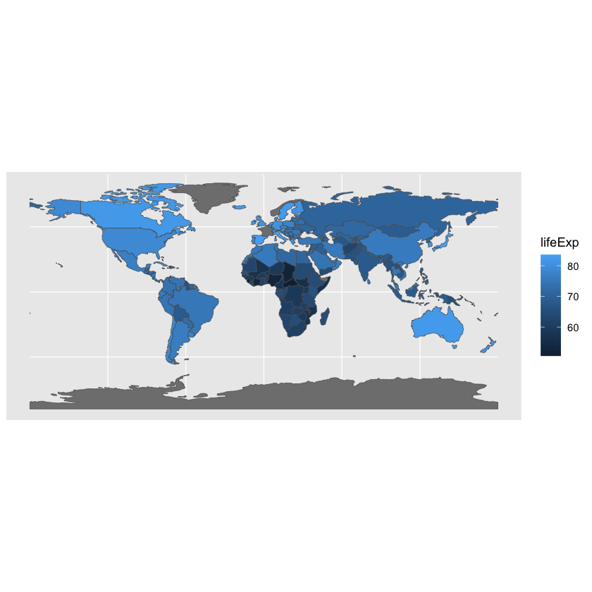
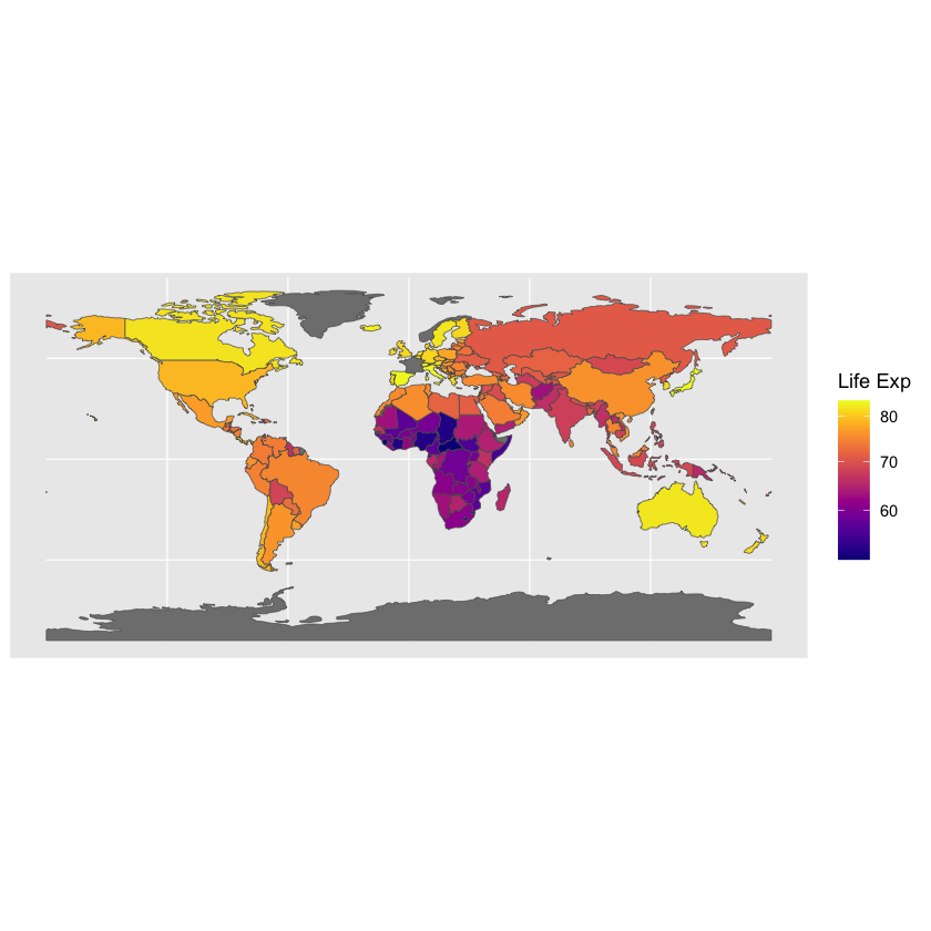
If you look at world, it also provides life expectancy estimates from 2014 (World Bank). The data set is tidy, with one row corresponding to one country. We’ll use our known ggplot2 way of filling things in.
Code
library(ggplot2)library(sf)library(spData)# ggplot(data = world) + geom_sf() # a special geometry for plotting mapsggplot(data = spData::world) +geom_sf(aes(fill = lifeExp)) # a special geometry for plotting mapsggplot(data = spData::world) +geom_sf(aes(fill = lifeExp)) +# a special geometry for plotting maps viridis::scale_fill_viridis('Life Exp', option='plasma', trans='sqrt', labels = scales::label_number_si())
Example: another choropleth
Code
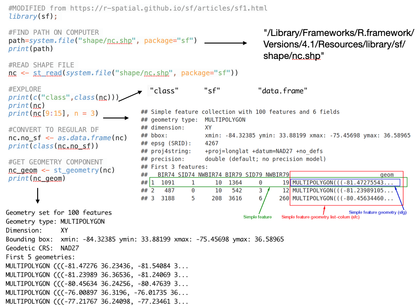
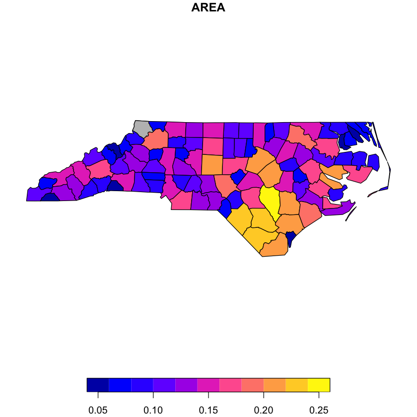
#MODIFIED from https://r-spatial.github.io/sf/articles/sf1.htmllibrary(sf); #FIND PATH ON COMPUTER path=system.file("shape/nc.shp", package="sf")# print(path)#READ SHAPE FILE nc <-st_read(system.file("shape/nc.shp", package="sf"))#EXPLORE# print(c("class",class(nc)))# print(nc)# print(nc[9:15], n = 3)#CONVERT TO REGULAR DFnc.no_sf <-as.data.frame(nc)# print(class(nc.no_sf))#GET GEOMETRY COMPONENT nc_geom <-st_geometry(nc)# print(nc_geom)#SF PLOTING FEATURE: EXAMPLE-1# par(mar = c(0,0,1,0))# reset = FALSE: we want to add to a plot with a legendplot(nc[1], reset =FALSE) plot(nc[1,1], col ='grey', add =TRUE)# #SF PLOTING FEATURE: EXAMPLE-2:# par(mar = c(0,0,1,0))# (w <- which(sapply(nc_geom, length) > 1))# ## [1] 4 56 57 87 91 95# plot(nc[w,1], col = 2:7)
Reading layer `nc' from data source
  `/Library/Frameworks/R.framework/Versions/4.2/Resources/library/sf/shape/nc.shp'
  using driver `ESRI Shapefile'
Simple feature collection with 100 features and 14 fields
Geometry type: MULTIPOLYGON
Dimension:     XY
Bounding box:  xmin: -84.32385 ymin: 33.88199 xmax: -75.45698 ymax: 36.58965
Geodetic CRS:  NAD27
R: Leaflet
The easiest ways to overlay data on street maps is with the leaflet package.
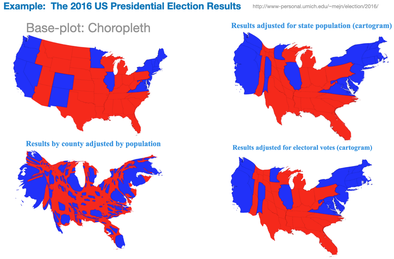
A cartogram is a map in which the geometry of regions is distorted in order to convey the information of an alternate variable. The region area will be inflated or deflated according to its value.
Start with a basic plot
Distort geometry based on chosen variable
Add color and now you have both a choropleth and a cartogram