[1] ‘1.8.0’[1] ‘0.6.1’From a first app to a published dashboard, all in R
Everything is in the lecture folder:
shiny-lecture/
├── shiny-lecture.ipynb        <- these notes
├── apps/
│   ├── 01-hello-shiny/        <- first app
│   ├── 02-mpg-explorer/       <- more widgets, more reactivity
│   ├── 03-hello-bslib/        <- first dashboard
│   └── 04-mpg-dashboard/      <- final product
└── images/Here are nine slides for the front of the lecture. Each cell starts with a ## header, so you can split them into separate notebook cells where you like.
One small terminology point: when you run an app locally, Shiny starts a real web server, a small program running on your own computer, rather than a “virtual” one. The slides call it a “local server,” which keeps the idea you wanted.
# How the Web Works: Clients and Servers

The big picture behind every web app

## Clients and servers

Every time you use the web, two sides are talking:

- **Client:** the program that *asks* for something (usually your web browser)
- **Server:** the program that *answers* (sends back a page, data, or a result)

**Restaurant analogy**

| Restaurant | Web |
|---|---|
| Customer places an order | Browser sends a **request** |
| Kitchen prepares the food | Server does the work |
| Waiter brings the plate | Server sends a **response** |

- You never see the kitchen, only the plate
- Each click, search, or slider move can be a new request

## A server is a program, not just a machine

- "Server" often means a big computer in a data center, but strictly it is **software that listens for requests and answers them**
- Any computer can run a server, **including your laptop**
- One computer can run many servers at once

**Examples**

- Google's servers answer searches
- Canvas's servers send your grades and assignments
- Your laptop running a Shiny app: also a server

## Client-side vs. server-side tools

**Where does the work happen?**

| | Client-side | Server-side |
|---|---|---|
| Runs on | The viewer's browser | A server somewhere else |
| Examples | Plotly charts, Quarto websites, JavaScript | Shiny, Google search, online banking |
| Data | Sent to the browser in full | Stays on the server |
| Needs a running server? | No, just files to download | Yes, always on |
| Good for | Static sites, light interactivity | Live data, big data, computation, privacy |

- **Client-side:** the server hands over the files once, then your browser does everything
- **Server-side:** the browser keeps asking the server to do new work

## IP addresses: how computers find each other

- Every device on a network has an **IP address**, like a mailing address for computers
- Example: `142.250.80.46` (one of Google's servers)
- Names like `google.com` are translated into IP addresses for you, like looking up a phone number in a contact list

**Two special kinds**

- **Public IP:** reachable from the internet (a website's server)
- **Private IP:** only reachable inside your home or campus network (for example `192.168.1.25`)

## Ports: which program on the computer?

- One computer can run many servers at once, so an IP address alone is not enough
- A **port** is a numbered door on that computer, and each server listens at its own door

**Analogy:** the IP address is the apartment building, the port is the apartment number

| Port | Typical use |
|---|---|
| 80 | Regular websites (`http`) |
| 443 | Secure websites (`https`) |
| 8080, 3838, random numbers | Development servers, like a local Shiny app |

A full address looks like this: `http://142.250.80.46:443`

## localhost: your computer talking to itself

- **`localhost`** is a special name that always means **"this computer"**
- Its IP address is always **`127.0.0.1`**
- Requests to localhost never leave your machine; there is no internet involved
- Other people **cannot** open your localhost address, because on their computer it points to *their* machine

> `localhost` is like writing "me" as the address on a letter: it always comes back to you.

## Running a Shiny app locally

When you click **Run App**, R does three things:

1. Starts a small **web server** inside your R session
2. Picks a **port** and listens on `127.0.0.1`
3. Opens your browser (the **client**) at that address

```
Listening on http://127.0.0.1:4321
```

| Piece | Who plays it |
|---|---|
| Client | Your web browser |
| Server | Your R session |
| Address | `127.0.0.1` (localhost) |
| Port | `4321` (changes each run unless you choose one) |

- Client and server are on the **same computer**, but they still talk over the web, exactly like a real website
- This is why your R console is busy: it is serving the app

## Local vs. deployed

**Local (today)**

- The server is your laptop, at `127.0.0.1`
- Only you can open the app
- It stops when you close R or your laptop

**Deployed (end of lecture)**

- The server is an always-on computer with a public address
- Anyone with the link can open the app, for example `https://your-name.shinyapps.io/my-app/`
- Same app code, it just lives on a different server

> Deploying = moving the server from your laptop to a computer the whole internet can reach.
The “Local vs. deployed” slide sets up the deployment section at the end, so you can point back to it there.
Install once (from the R console):
Then confirm the versions:
app.R file will also prompt you to install Shiny if it is missingBuild, run, and understand your first interactive app
Common uses
Shiny ships with built-in example apps. Run these in your R console:
library(shiny)
runExample()               # lists all examples
runExample("01_hello")     # a slider that controls a histogram
runExample("06_tabsets") # inputs plus tabsEvery app has exactly two parts plus one line that connects them.
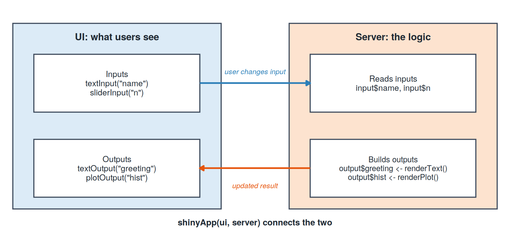
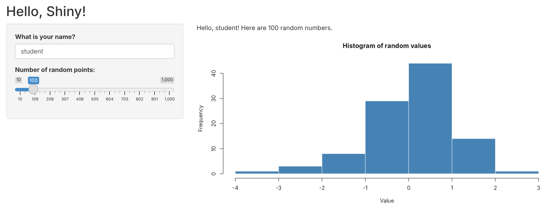
shinyApp(ui, server): launches the appCreate a folder 01-hello-shiny/ with one file named exactly app.R:
apps/01-hello-shiny/app.R
# ------------------------------------------------------------
# App 1: Hello, Shiny!
# The smallest useful Shiny app: two inputs, two outputs.
#
# Run it:
#   RStudio:       open this file and click "Run App"
#   R console:     shiny::runApp("01-hello-shiny")
#   Command line:  Rscript -e 'shiny::runApp("01-hello-shiny", launch.browser = TRUE)'
# ------------------------------------------------------------

library(shiny)

# ---- UI: what the user sees ---------------------------------
ui <- fluidPage(
  titlePanel("Hello, Shiny!"),

  sidebarLayout(
    sidebarPanel(
      textInput("name", "What is your name?", value = "student"),
      sliderInput("n", "Number of random points:",
                  min = 10, max = 1000, value = 100)
    ),

    mainPanel(
      textOutput("greeting"),
      plotOutput("hist")
    )
  )
)

# ---- Server: the logic behind the page ----------------------
server <- function(input, output, session) {

  # Re-runs whenever input$name changes
  output$greeting <- renderText({
    paste0("Hello, ", input$name, "! Here are ", input$n, " random numbers.")
  })

  # Re-runs whenever input$n changes
  output$hist <- renderPlot({
    hist(rnorm(input$n),
         col = "steelblue", border = "white",
         main = "Histogram of random values", xlab = "Value")
  })
}

# ---- Connect the two ----------------------------------------
shinyApp(ui = ui, server = server)App 1: Hello, Shiny!
One-file app (recommended)
01-hello-shiny/
└── app.R          # ui, server, and shinyApp() together
Two-file app (older style, still common online)
my-app/
├── ui.R           # just the ui
└── server.R       # just the server function
Rules of thumb
app.R (or ui.R + server.R) for Run App to workapp.RStop it: click the red stop sign in the console, or press Esc
Tip: after editing app.R, just click Reload App. No need to restart.
The same thing, typed instead of clicked:
library(shiny)

# Run an app folder (path is relative to your working directory)
runApp("apps/01-hello-shiny")

# Open in your browser and pick a port
runApp("apps/01-hello-shiny", launch.browser = TRUE, port = 8080)Listening on http://127.0.0.1:8080No editor needed. From a terminal (Git Bash on Windows, Terminal on macOS):
# go to the lecture folder first
cd shiny-lecture

# run and open the browser automatically
Rscript -e 'shiny::runApp("apps/01-hello-shiny", launch.browser = TRUE)'

# run on a fixed port, then visit http://127.0.0.1:8080
Rscript -e 'shiny::runApp("apps/01-hello-shiny", port = 8080)'Ctrl + C in the terminalRscript not found? R is not on your PATH. Use the full path to Rscript, or run from RStudio’s Terminal tab.| Where | How | Stop |
|---|---|---|
| RStudio | Open app.R, click Run App |
Esc or stop sign |
| VS Code / Positron | Shiny extension, Run Shiny App button | Stop button |
| R console | shiny::runApp("folder") |
Esc or Ctrl + C |
| Terminal | Rscript -e 'shiny::runApp("folder")' |
Ctrl + C |
Key idea: every option starts the same thing, a small web server powered by your R session. While it runs, that R session is busy serving the app.
That is also why these notes show app code as text: running an app inside a notebook would block the notebook.
| Function | Widget | Value in input$id |
|---|---|---|
sliderInput() |
slider (single value or range) | number(s) |
selectInput() |
dropdown menu | text |
textInput() |
text box | text |
numericInput() |
number box | number |
checkboxInput() |
single checkbox | TRUE / FALSE |
checkboxGroupInput() |
several checkboxes | vector of choices |
radioButtons() |
pick exactly one | text |
dateInput() |
calendar | date |
actionButton() |
button | click count |
Every input starts with the same two arguments:
Run a UI function in the console and you get web page code back:
<div class="form-group shiny-input-container">
  <label class="control-label" id="name-label" for="name">What is your name?</label>
  <input id="name" type="text" class="shiny-input-text form-control" value=""/>
</div>Outputs always come in pairs: a placeholder in the UI and a render function in the server.
| UI placeholder | Server render function | Shows |
|---|---|---|
plotOutput("id") |
renderPlot({ ... }) |
plots (base R or ggplot2) |
tableOutput("id") |
renderTable({ ... }) |
data frames |
textOutput("id") |
renderText({ ... }) |
text |
verbatimTextOutput("id") |
renderPrint({ ... }) |
console-style output |
uiOutput("id") |
renderUI({ ... }) |
UI built on the fly |
input$ and output$Inside the server:
input$<id>output$<id> <- render...()plotOutput("histogram") but output$hist. Nothing appears, and there is no error.output$hist <- hist(...) fails; it must be renderPlot({ hist(...) })input$n only works inside render*(), reactive(), or observe*()read.csv("data.csv") fails because the file is not inside the app folderDebugging tip: add print(input$n) inside a render function and watch the console.
When an input changes, anything that uses it updates automatically.
In App 1, Shiny tracks these dependencies:
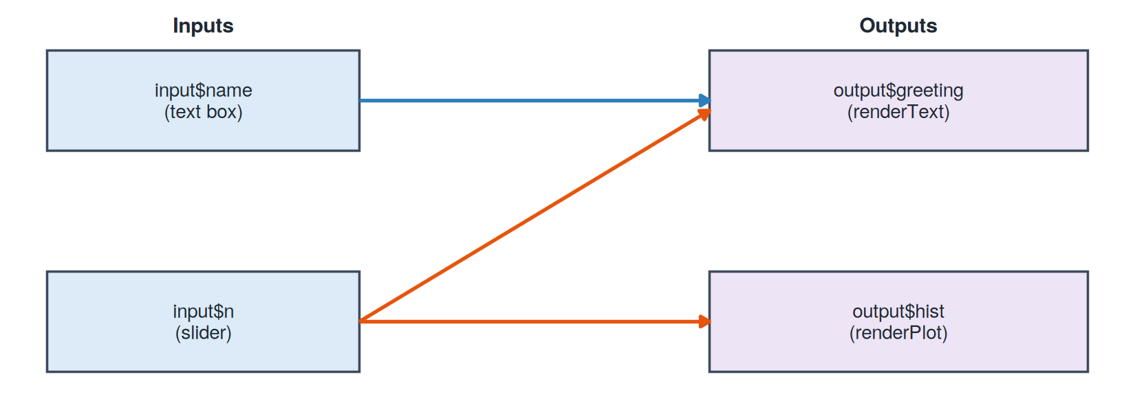
Shiny’s reactive values can be explored right in the console:
total remembers its recipe, not just its valuereactiveVal()reactive(): compute once, use everywhereProblem: several outputs need the same filtered data.
# Without reactive(): the filter runs 3 times
output$plot  <- renderPlot({ data <- filter(mpg, class == input$class); ... })
output$table <- renderTable({ data <- filter(mpg, class == input$class); ... })
output$count <- renderText({ data <- filter(mpg, class == input$class); ... })
# With reactive(): write it once, reuse it
filtered <- reactive({
filter(mpg, class == input$class)
})
output$plot <- renderPlot({ ggplot(filtered(), ...) })
output$table <- renderTable({ filtered() })
output$count <- renderText({ nrow(filtered()) })filtered()input$class changes, and caches the result| manufacturer | model | displ | year | cyl | trans | drv | cty | hwy | fl | class |
|---|---|---|---|---|---|---|---|---|---|---|
| audi | a4 | 1.8 | 1999 | 4 | auto(l5) | f | 18 | 29 | p | compact |
| audi | a4 | 1.8 | 1999 | 4 | manual(m5) | f | 21 | 29 | p | compact |
| audi | a4 | 2.0 | 2008 | 4 | manual(m6) | f | 20 | 31 | p | compact |
| audi | a4 | 2.0 | 2008 | 4 | auto(av) | f | 21 | 30 | p | compact |
| audi | a4 | 2.8 | 1999 | 6 | auto(l5) | f | 16 | 26 | p | compact |
| audi | a4 | 2.8 | 1999 | 6 | manual(m5) | f | 18 | 26 | p | compact |
| audi | a4 | 3.1 | 2008 | 6 | auto(av) | f | 18 | 27 | p | compact |
| audi | a4 quattro | 1.8 | 1999 | 4 | manual(m5) | 4 | 18 | 26 | p | compact |
| audi | a4 quattro | 1.8 | 1999 | 4 | auto(l5) | 4 | 16 | 25 | p | compact |
| audi | a4 quattro | 2.0 | 2008 | 4 | manual(m6) | 4 | 20 | 28 | p | compact |
Key: displ engine size (L), cyl cylinders, trans transmission, drv drive (f = front, r = rear, 4 = 4WD), cty / hwy city / highway MPG, fl fuel type (p = premium)
A regular (non-dashboard) app that uses more of Shiny’s toolbox.
App 2: MPG Explorer
Reading a real Shiny app from top to bottom
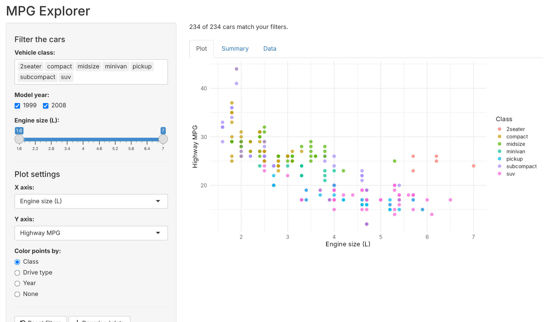
What the app does: lets users filter the mpg cars and explore them as a plot, a summary, or a raw table.
How the file is organized
| Section | Lines | Job |
|---|---|---|
| Setup | top | Load packages, prepare data and labels |
| UI | ui <- fluidPage(...) |
Layout, inputs, output placeholders |
| Server | server <- function(...) |
Filter data, build outputs, handle buttons |
| Launch | shinyApp(ui, server) |
Start the app |
Reading tip: read the UI first to see what users can do, then the server to see what happens when they do it.
library(shiny)
library(ggplot2)
library(dplyr)

cars <- mpg

num_vars <- c(
  "Engine size (L)" = "displ",
  "City MPG"        = "cty",
  "Highway MPG"     = "hwy",
  "Cylinders"       = "cyl"
)ui and server runs once, when the app startsnum_vars is a named vector:
"hwy"ui <- fluidPage(
titlePanel("MPG Explorer"),
sidebarLayout(
sidebarPanel( ...inputs... ),
mainPanel( ...outputs... )
)
)┌──────────────────────────────────────────────┐
│ MPG Explorer (titlePanel) │
├───────────────┬──────────────────────────────┤
│ sidebarPanel │ mainPanel │
│ │ │
│ filters │ "109 of 234 cars match..." │
│ plot settings │ [ Plot | Summary | Data ] │
│ buttons │ │
└───────────────┴──────────────────────────────┘h4() adds a small heading, hr() a divider line, br() a blank lineselectInput("class", "Vehicle class:",
choices = sort(unique(cars$class)),
selected = sort(unique(cars$class)),
multiple = TRUE)
checkboxGroupInput("year", "Model year:",
choices = c(1999, 2008), selected = c(1999, 2008))
sliderInput("displ", "Engine size (L):",
min = min(cars$displ), max = max(cars$displ),
value = range(cars$displ), step = 0.1)| Input | Widget | What input$... holds |
|---|---|---|
input$class |
multi-select dropdown | one or more classes, e.g. c("suv", "compact") |
input$year |
checkboxes | one or both years |
input$displ |
range slider (two handles) | two numbers: c(low, high) |
choices and selected come from the data, so nothing is typed by handvalue two numbers turns a slider into a range sliderselectInput("x", "X axis:", choices = num_vars, selected = "displ")
selectInput("y", "Y axis:", choices = num_vars, selected = "hwy")
radioButtons("color", "Color points by:",
choices = c("Class" = "class", "Drive type" = "drv",
"Year" = "year", "None" = "none"))
actionButton("reset", "Reset filters", icon = icon("rotate-left"))
downloadButton("download", "Download data")input$x and input$y hold column names as text, like "hwy"input$color holds "class", "drv", "year", or "none"input$reset counts clicks: 0, 1, 2, …output$downloadmainPanel(
textOutput("count"),
tabsetPanel(
tabPanel("Plot", plotOutput("scatter", height = "450px")),
tabPanel("Summary", tableOutput("summary")),
tabPanel("Data", tableOutput("table"))
)
)tabsetPanel() stacks the three views behind clickable tabs"scatter" here, output$scatter therefiltered <- reactive({
cars |>
filter(class %in% input$class,
year %in% input$year,
displ >= input$displ[1],
displ <= input$displ[2])
})%in% keeps a row if its value matches any of the selected choicesinput$displ[1] is the slider’s low end and input$displ[2] its high endfiltered(), so the filtering is written once and runs once per changeoutput$count <- renderText({
paste(nrow(filtered()), "of", nrow(cars), "cars match your filters.")
})output$scatter <- renderPlot({
validate(need(nrow(filtered()) > 0, "No cars match these filters."))
p <- ggplot(filtered(), aes(x = .data[[input$x]], y = .data[[input$y]]))
...
})validate(need(...)): if no cars are left, show a friendly message instead of an error.data[[input$x]]: input$x is text like "hwy", and this tells ggplot “use the column with this name”if / else adds colored points, or plain blue points when “None” is pickednames(num_vars)[num_vars == input$x] looks up the friendly axis label: "hwy" becomes “Highway MPG”output$summary <- renderTable({
filtered() |>
group_by(class) |>
summarise(cars = n(),
avg_city_mpg = mean(cty),
avg_hwy_mpg = mean(hwy)) |>
arrange(desc(avg_hwy_mpg))
}, digits = 1)
output$table <- renderTable({
filtered() |>
select(manufacturer, model, year, class, displ, cyl, drv, cty, hwy)
})renderTable({ }) around it, and filtered() instead of mpgobserveEvent(input$reset, {
updateSelectInput(session, "class", selected = sort(unique(cars$class)))
updateCheckboxGroupInput(session, "year", selected = c(1999, 2008))
updateSliderInput(session, "displ", value = range(cars$displ))
})observeEvent(input$reset, { ... }) means “every time the button is clicked, run this”update*Input() changes a widget from the server, and session says which user’s page to changefiltered(), so every output updates on its ownoutput$download <- downloadHandler(
filename = function() "mpg-filtered.csv",
content = function(file) write.csv(filtered(), file, row.names = FALSE)
)filename: what the downloaded file is calledcontent: how to write it, which here means saving the current filtered() data as a CSVThe user unchecks 1999:
input$year changes from c(1999, 2008) to 2008filtered() re-runs: now only 2008 carsfiltered() updates: the count, plot, summary, and tableThe user changes the X axis:
input$x changesinput$xfiltered() does not re-run, since no filter changedShiny only redoes the work that depends on what changed.
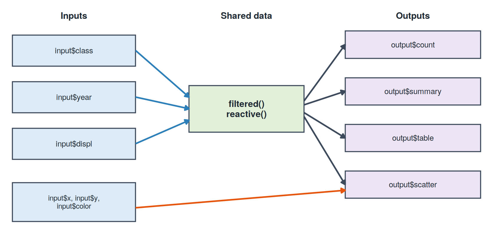
reactive(), which feeds every outputRespond to a button with observeEvent() (for side effects, not outputs)
Show a friendly message instead of an error with validate()
Let users download the data with downloadHandler()
output$download <- downloadHandler(
filename = function() "mpg-filtered.csv",
content = function(file) write.csv(filtered(), file, row.names = FALSE)
)Organize views with tabsetPanel()
apps/02-mpg-explorer/app.R
# ------------------------------------------------------------
# App 2: MPG Explorer
# A classic Shiny app (not a dashboard) that shows off more widgets
# and the key reactivity tools:
# - several input types (select, checkbox group, slider, radio)
# - reactive() to share one filtered dataset across outputs
# - tabsetPanel() for multiple views
# - observeEvent() + update*Input() for a "Reset" button
# - downloadHandler() to export the filtered data
#
# Run it: shiny::runApp("02-mpg-explorer")
# ------------------------------------------------------------
library(shiny)
library(ggplot2)
library(dplyr)
# mpg ships with ggplot2: 234 cars from 1999 and 2008
cars <- mpg
# Friendly labels for the numeric variables users can plot
num_vars <- c(
"Engine size (L)" = "displ",
"City MPG" = "cty",
"Highway MPG" = "hwy",
"Cylinders" = "cyl"
)
# ---- UI ------------------------------------------------------
ui <- fluidPage(
titlePanel("MPG Explorer"),
sidebarLayout(
sidebarPanel(
h4("Filter the cars"),
selectInput("class", "Vehicle class:",
choices = sort(unique(cars$class)),
selected = sort(unique(cars$class)),
multiple = TRUE),
checkboxGroupInput("year", "Model year:",
choices = c(1999, 2008),
selected = c(1999, 2008),
inline = TRUE),
sliderInput("displ", "Engine size (L):",
min = min(cars$displ), max = max(cars$displ),
value = range(cars$displ), step = 0.1),
hr(),
h4("Plot settings"),
selectInput("x", "X axis:", choices = num_vars, selected = "displ"),
selectInput("y", "Y axis:", choices = num_vars, selected = "hwy"),
radioButtons("color", "Color points by:",
choices = c("Class" = "class", "Drive type" = "drv",
"Year" = "year", "None" = "none"),
selected = "class"),
hr(),
actionButton("reset", "Reset filters", icon = icon("rotate-left")),
downloadButton("download", "Download data")
),
mainPanel(
textOutput("count"),
br(),
tabsetPanel(
tabPanel("Plot", plotOutput("scatter", height = "450px")),
tabPanel("Summary", tableOutput("summary")),
tabPanel("Data", tableOutput("table"))
)
)
)
)
# ---- Server --------------------------------------------------
server <- function(input, output, session) {
# One reactive expression feeds every output below.
# It re-runs only when one of the filter inputs changes.
filtered <- reactive({
  cars |>
    filter(class %in% input$class,
           year  %in% input$year,
           displ >= input$displ[1],
           displ <= input$displ[2])
})
output$count <- renderText({
  paste(nrow(filtered()), "of", nrow(cars), "cars match your filters.")
})
output$scatter <- renderPlot({
# validate() shows a friendly message instead of an error
validate(need(nrow(filtered()) > 0, "No cars match these filters."))
p <- ggplot(filtered(), aes(x = .data[[input$x]], y = .data[[input$y]]))
if (input$color == "none") {
p <- p + geom_point(size = 3, alpha = 0.7, color = "steelblue")
} else {
color_labels <- c(class = "Class", drv = "Drive type", year = "Year")
p <- p +
geom_point(aes(color = factor(.data[[input$color]])),
size = 3, alpha = 0.7) +
labs(color = color_labels[[input$color]])
}
p +
labs(x = names(num_vars)[num_vars == input$x],
y = names(num_vars)[num_vars == input$y]) +
theme_minimal(base_size = 15)
})
output$summary <- renderTable({
  filtered() |>
    group_by(class) |>
    summarise(cars = n(),
              avg_city_mpg = mean(cty),
              avg_hwy_mpg  = mean(hwy)) |>
    arrange(desc(avg_hwy_mpg))
}, digits = 1)

output$table <- renderTable({
  filtered() |>
    select(manufacturer, model, year, class, displ, cyl, drv, cty, hwy)
})
# observeEvent() runs code for its side effect (here: changing inputs)
observeEvent(input$reset, {
  updateSelectInput(session, "class", selected = sort(unique(cars$class)))
  updateCheckboxGroupInput(session, "year", selected = c(1999, 2008))
  updateSliderInput(session, "displ", value = range(cars$displ))
})
output$download <- downloadHandler(
  filename = function() "mpg-filtered.csv",
  content  = function(file) write.csv(filtered(), file, row.names = FALSE)
)
}
shinyApp(ui, server)Get the plot working as plain R, then swap in the inputs:
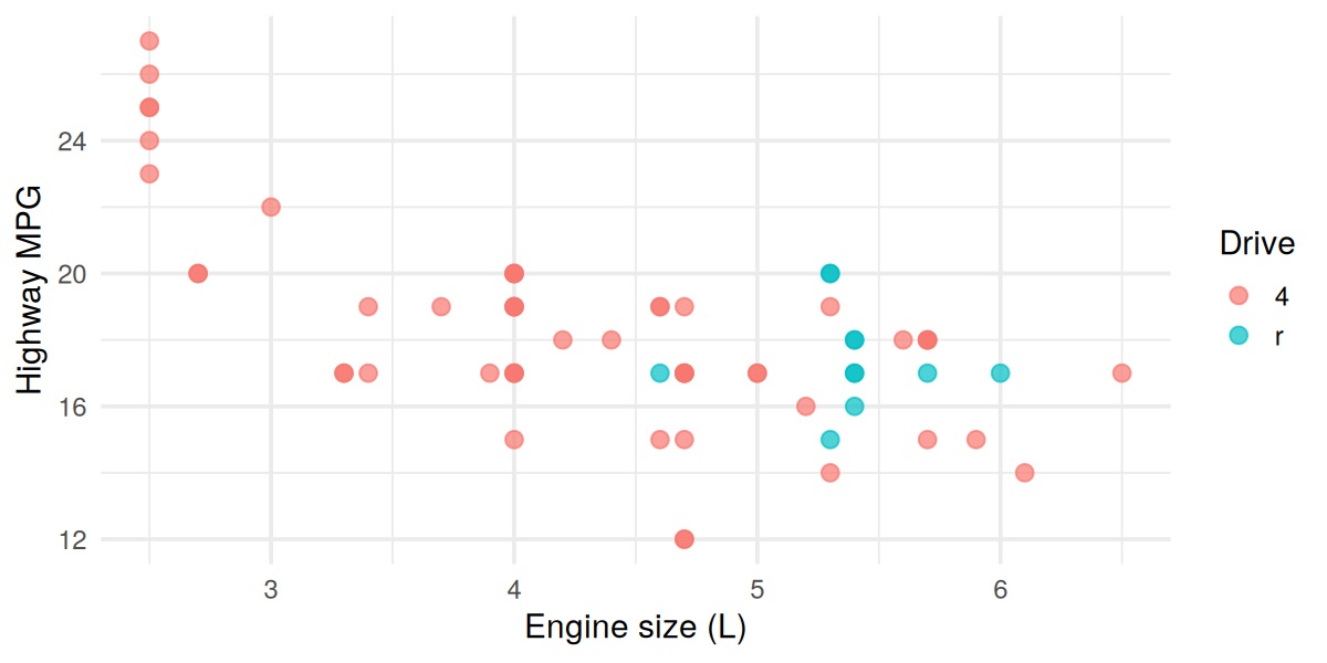
renderPlot({ ... }) and replace chosen_class with input$classThe ideas behind dashboards, and when they need a server
A dashboard is a single screen showing the most important information about something, at a glance.
Everyday examples
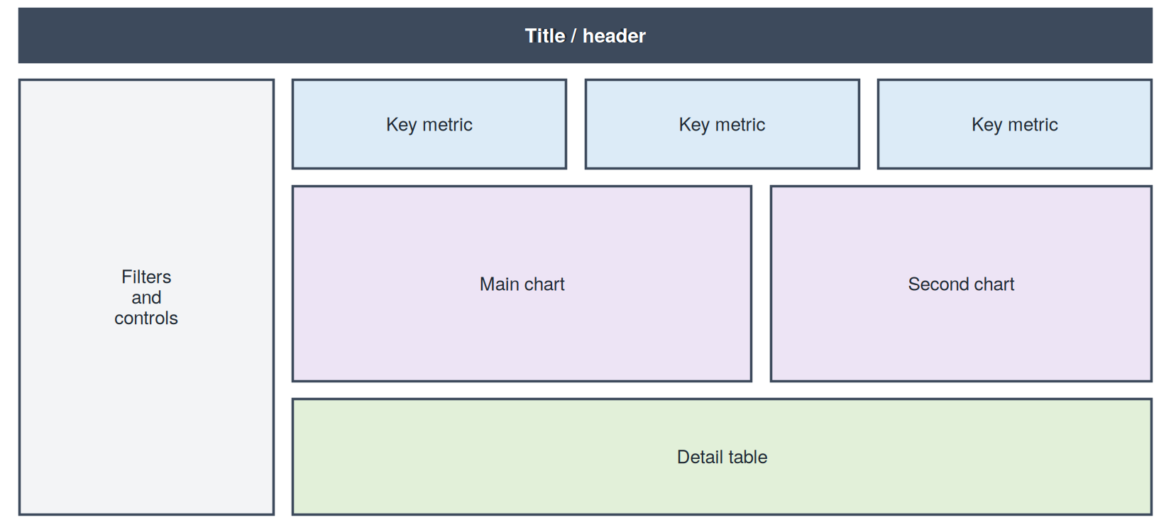
displ vs hwy)Report
Dashboard
You can already make interactive charts without Shiny (for example with Plotly or htmlwidgets). So why run R behind the page?
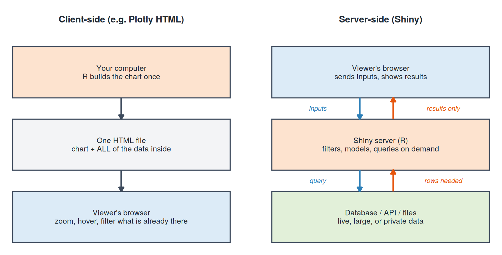
Data
Computation
Security
Two-way apps
Client-side (Plotly, htmlwidgets)
Server-side (Shiny)
Rule of thumb: if a static chart answers the question, use a static chart. Reach for Shiny when users need the app to compute something new.
Same Shiny engine, a modern dashboard body
What changes, what stays the same
render*() functions, reactive(), the whole serverShiny is the engine. bslib is the car body around it.
Note: you will see shinydashboard in older tutorials. Same idea, older package, different function names (dashboardPage(), box(), valueBox()).
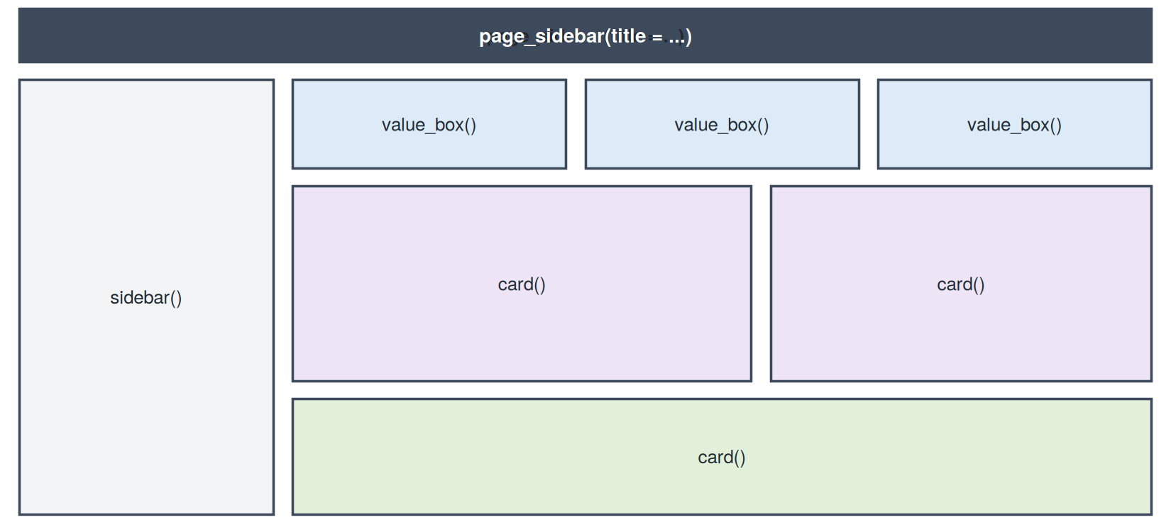
| Function | Role |
|---|---|
page_sidebar() |
The whole page: title bar, sidebar, main area |
sidebar() |
Collapsible panel for inputs |
value_box() |
Headline number with an optional icon |
card() + card_header() |
A bordered panel for a chart or table |
layout_columns() |
Places items side by side in a row |
bs_theme() |
Colors, fonts, and ready-made themes |
Classic Shiny (App 1)
App 3 uses made-up data, created right inside app.R:
set.seed(42)
coffee <- data.frame(
  day      = 1:60,
  visitors = round(120 + 2 * (1:60) + rnorm(60, sd = 15))
)
What the code does
day: days 1 through 60 (about two months)visitors: starts around 120, grows by about 2 visitors per day, plus random day-to-day noisernorm(60, sd = 15): adds realistic ups and downsset.seed(42): makes the “random” numbers the same every time, so everyone sees identical resultsFirst few rows
| day | visitors |
|---|---|
| 1 | 143 |
| 2 | 116 |
| 3 | 131 |
| 4 | 137 |
| 5 | 136 |
Quick summary (all 60 days)
| Statistic | Value |
|---|---|
| Fewest visitors in a day | 116 |
| Most visitors in a day | 250 |
| Average per day | about 181 |
| Total visitors | 10,836 |
In the dashboard
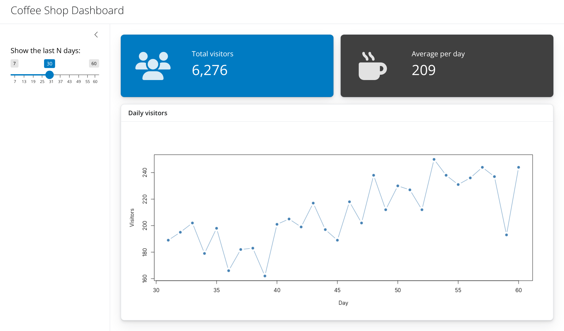
The smallest possible dashboard: toy data, one slider, two value boxes, one chart.
apps/03-hello-bslib/app.R
# ------------------------------------------------------------
# App 3: Hello, bslib!
# The smallest possible dashboard: a sidebar, two value boxes,
# and one chart card. Uses made-up (toy) data.
#
# Same Shiny engine as App 1. Only the UI functions change:
#   fluidPage()  ->  page_sidebar()
#   panels       ->  card() and value_box()
#
# Run it:  shiny::runApp("03-hello-bslib")
# ------------------------------------------------------------

library(shiny)
library(bslib)

# Toy data: daily visitors to a coffee shop for 60 days
set.seed(42)
coffee <- data.frame(
  day      = 1:60,
  visitors = round(120 + 2 * (1:60) + rnorm(60, sd = 15))
)

# ---- UI ------------------------------------------------------
ui <- page_sidebar(
  title = "Coffee Shop Dashboard",

  sidebar = sidebar(
    sliderInput("days", "Show the last N days:",
                min = 7, max = 60, value = 30)
  ),

  # Two headline numbers side by side
  layout_columns(
    value_box(
      title = "Total visitors",
      value = textOutput("total"),
      showcase = icon("users"),
      theme = "primary"
    ),
    value_box(
      title = "Average per day",
      value = textOutput("average"),
      showcase = icon("mug-hot"),
      theme = "secondary"
    )
  ),

  # One chart in a card
  card(
    card_header("Daily visitors"),
    plotOutput("trend")
  )
)

# ---- Server --------------------------------------------------
server <- function(input, output, session) {

  recent <- reactive({
    tail(coffee, input$days)
  })

  output$total   <- renderText(format(sum(recent()$visitors), big.mark = ","))
  output$average <- renderText(round(mean(recent()$visitors)))

  output$trend <- renderPlot({
    plot(recent()$day, recent()$visitors, type = "b", pch = 19,
         col = "steelblue", xlab = "Day", ylab = "Visitors")
  })
}

shinyApp(ui, server)App 3: Hello, bslib!
value_box(
  title    = "Total visitors",       # small label
  value    = textOutput("total"),    # the big number (can be reactive)
  showcase = icon("users"),          # optional icon on the left
  theme    = "primary"               # color: primary, success, info, ...
)
value can be fixed text or a textOutput() that the server fills inicon() uses the free Font Awesome icon set; search names at fontawesome.comlayout_columns() to make a rowlayout_columns(
col_widths = c(7, 5), # widths out of 12
card(
full_screen = TRUE, # adds an "expand" button
card_header("Main chart"),
plotOutput("scatter")
),
card(
card_header("Second chart"),
plotOutput("bars")
)
)c(7, 5) means 7/12 and 5/12 of the widthfull_screen = TRUE lets users enlarge a card, which is great for presentationspage_sidebar() stack vertically; layout_columns() puts them side by sideChange the whole look with one argument:
ui <- page_sidebar(
  title = "My dashboard",
  theme = bs_theme(bootswatch = "flatly", primary = "#2C7FB8"),
  ...
)
bootswatch offers ready-made themes: "flatly", "minty", "darkly", "lux", "sandstone", …bs_theme(primary = ..., base_font = ...)bs_themer() as the first line of your server function, then pick from a menu while the app runsEverything combined into one polished app
mpgShips with ggplot2, so there is nothing to download.
| manufacturer | model | displ | year | cyl | trans | drv | cty | hwy | fl | class |
|---|---|---|---|---|---|---|---|---|---|---|
| <chr> | <chr> | <dbl> | <int> | <int> | <chr> | <chr> | <int> | <int> | <chr> | <chr> |
| audi | a4 | 1.8 | 1999 | 4 | auto(l5) | f | 18 | 29 | p | compact |
| audi | a4 | 1.8 | 1999 | 4 | manual(m5) | f | 21 | 29 | p | compact |
| audi | a4 | 2.0 | 2008 | 4 | manual(m6) | f | 20 | 31 | p | compact |
| audi | a4 | 2.0 | 2008 | 4 | auto(av) | f | 21 | 30 | p | compact |
| audi | a4 | 2.8 | 1999 | 6 | auto(l5) | f | 16 | 26 | p | compact |
| audi | a4 | 2.8 | 1999 | 6 | manual(m5) | f | 18 | 26 | p | compact |
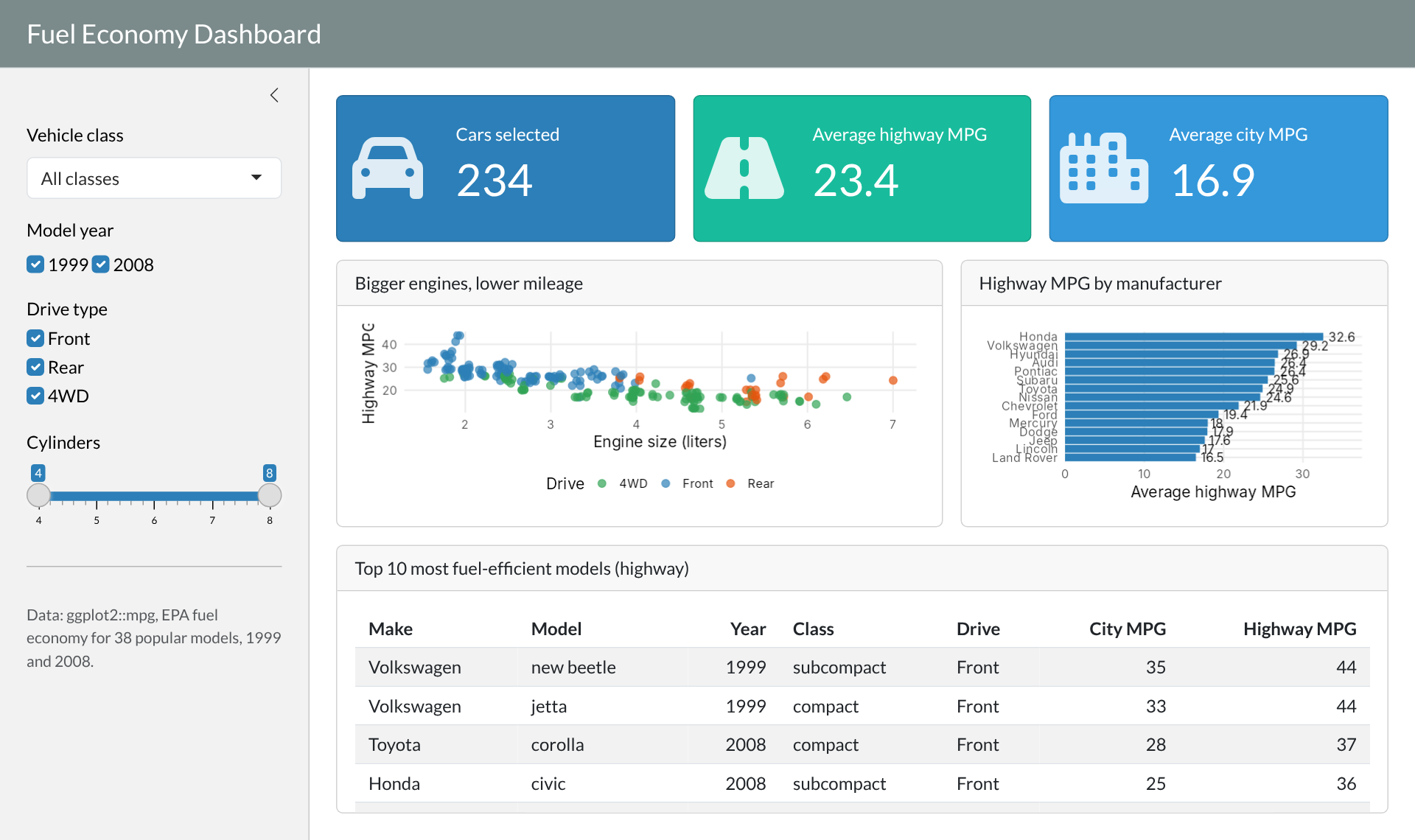
manufacturer, class, drv (drive type), year, cylcty and hwy (city and highway miles per gallon), displ (engine size)Audience: someone shopping for a fuel-efficient car
Questions the dashboard should answer
Map questions to building blocks
| Question | Building block |
|---|---|
| 1, 2 | Three value boxes |
| 3 | Scatter plot card |
| 4 | Bar chart card |
| 5 | Top 10 table card |
| “what I am looking for” | Sidebar filters: class, year, drive, cylinders |
App 4: Fuel Economy Dashboard
Clean labels once, at the top of app.R, outside the server:
| drive | n |
|---|---|
| <chr> | <int> |
| 4WD | 103 |
| Front | 106 |
| Rear | 25 |
The skeleton, with details removed:
ui <- page_sidebar(
  title = "Fuel Economy Dashboard",
  theme = bs_theme(bootswatch = "flatly", primary = "#2C7FB8"),

  sidebar = sidebar(
    selectInput("class", "Vehicle class", ...),
    checkboxGroupInput("year", "Model year", ...),
    checkboxGroupInput("drive", "Drive type", ...),
    sliderInput("cyl", "Cylinders", ...)
  ),

  layout_columns(                                       # row 1
    value_box("Cars selected",       textOutput("n_cars"),  ...),
    value_box("Average highway MPG", textOutput("avg_hwy"), ...),
    value_box("Average city MPG",    textOutput("avg_cty"), ...)
  ),

  layout_columns(col_widths = c(7, 5),                  # row 2
    card(card_header("Bigger engines, lower mileage"), plotOutput("scatter")),
    card(card_header("Highway MPG by manufacturer"),   plotOutput("by_make"))
  ),

  card(card_header("Top 10 most fuel-efficient models"),  # row 3
       tableOutput("top10"))
)filtered <- reactive({
data <- cars |>
filter(year %in% input$year,
drive %in% input$drive,
cyl >= input$cyl[1],
cyl <= input$cyl[2])
if (input$class != "All classes") {
data <- filter(data, class == input$class)
}
data
})filtered()input$cyl is a range slider, so it has two values: [1] and [2]# Value boxes: just a number
output$n_cars <- renderText(nrow(filtered()))
output$avg_hwy <- renderText(round(mean(filtered()$hwy), 1))
# Charts: normal ggplot code using filtered()
output$scatter <- renderPlot({
ggplot(filtered(), aes(displ, hwy, color = drive)) +
geom_jitter(size = 3, alpha = 0.7) +
labs(x = "Engine size (liters)", y = "Highway MPG")
})
# Table: normal dplyr code using filtered()
output$top10 <- renderTable({
filtered() |>
arrange(desc(hwy)) |>
slice_head(n = 10)
})Pattern: every output is ordinary R code wrapped in a render*() function, using filtered() instead of the raw data.
Ask while demoing: which input triggered which output? Why did the table change but not the page layout?
apps/04-mpg-dashboard/app.R
# ------------------------------------------------------------
# App 4: Fuel Economy Dashboard (final product)
# A polished but beginner-friendly bslib dashboard built on the
# mpg dataset from ggplot2.
#
# Structure:
# sidebar -> filters (inputs)
# value boxes -> headline numbers
# cards -> two charts and a table
# reactive() -> one filtered dataset shared by every output
#
# Run it: shiny::runApp("04-mpg-dashboard")
# ------------------------------------------------------------
library(shiny)
library(bslib)
library(ggplot2)
library(dplyr)
# ---- Data ----------------------------------------------------
cars <- mpg |>
mutate(
drive = recode(drv, "f" = "Front", "r" = "Rear", "4" = "4WD"),
make = tools::toTitleCase(manufacturer)
)
all_classes <- sort(unique(cars$class))
# ---- Theme ---------------------------------------------------
my_theme <- bs_theme(
version = 5,
bootswatch = "flatly",
primary = "#2C7FB8"
)
# Shared ggplot style so every chart looks consistent
theme_dash <- theme_minimal(base_size = 14) +
theme(panel.grid.minor = element_blank(),
legend.position = "bottom")
# ---- UI ------------------------------------------------------
ui <- page_sidebar(
title = "Fuel Economy Dashboard",
theme = my_theme,
sidebar = sidebar(
width = 280,
selectInput("class", "Vehicle class",
choices = c("All classes", all_classes),
selected = "All classes"),
checkboxGroupInput("year", "Model year",
choices = c(1999, 2008),
selected = c(1999, 2008),
inline = TRUE),
checkboxGroupInput("drive", "Drive type",
choices = c("Front", "Rear", "4WD"),
selected = c("Front", "Rear", "4WD")),
sliderInput("cyl", "Cylinders",
min = 4, max = 8, value = c(4, 8), step = 1),
hr(),
p(class = "text-muted small",
"Data: ggplot2::mpg, EPA fuel economy for 38 popular models, 1999 and 2008.")
),
# Row 1: headline numbers
layout_columns(
fill = FALSE,
value_box(
title = "Cars selected",
value = textOutput("n_cars"),
showcase = icon("car"),
theme = "primary"
),
value_box(
title = "Average highway MPG",
value = textOutput("avg_hwy"),
showcase = icon("road"),
theme = "success"
),
value_box(
title = "Average city MPG",
value = textOutput("avg_cty"),
showcase = icon("city"),
theme = "info"
)
),
# Row 2: two charts side by side
layout_columns(
col_widths = c(7, 5),
card(
full_screen = TRUE,
card_header("Bigger engines, lower mileage"),
plotOutput("scatter")
),
card(
full_screen = TRUE,
card_header("Highway MPG by manufacturer"),
plotOutput("by_make")
)
),
# Row 3: table of the most efficient cars
card(
card_header("Top 10 most fuel-efficient models (highway)"),
tableOutput("top10")
)
)
# ---- Server --------------------------------------------------
server <- function(input, output, session) {
# One filtered dataset, reused by every output
filtered <- reactive({
  data <- cars |>
    filter(year  %in% input$year,
           drive %in% input$drive,
           cyl   >= input$cyl[1],
           cyl   <= input$cyl[2])

  if (input$class != "All classes") {
    data <- filter(data, class == input$class)
  }
  data
})
# Friendly message when the filters remove every car
check_data <- function() {
validate(need(nrow(filtered()) > 0,
"No cars match these filters. Try widening them."))
}
# ---- Value boxes ----
output$n_cars <- renderText(nrow(filtered()))
output$avg_hwy <- renderText({
check_data()
round(mean(filtered()$hwy), 1)
})
output$avg_cty <- renderText({
check_data()
round(mean(filtered()$cty), 1)
})
# ---- Charts ----
output$scatter <- renderPlot({
check_data()
ggplot(filtered(), aes(displ, hwy, color = drive)) +
geom_jitter(size = 3, alpha = 0.7, width = 0.05, height = 0.3) +
scale_color_manual(values = c(Front = "#2C7FB8", Rear = "#E6550D",
`4WD` = "#31A354")) +
labs(x = "Engine size (liters)", y = "Highway MPG", color = "Drive") +
theme_dash
})
output$by_make <- renderPlot({
check_data()
filtered() |>
group_by(make) |>
summarise(hwy = mean(hwy)) |>
ggplot(aes(x = hwy, y = reorder(make, hwy))) +
geom_col(fill = "#2C7FB8") +
geom_text(aes(label = round(hwy, 1)), hjust = -0.2, size = 4) +
scale_x_continuous(expand = expansion(mult = c(0, 0.15))) +
labs(x = "Average highway MPG", y = NULL) +
theme_dash
})
# ---- Table ----
output$top10 <- renderTable({
check_data()
filtered() |>
arrange(desc(hwy), desc(cty)) |>
distinct(make, model, year, .keep_all = TRUE) |>
slice_head(n = 10) |>
transmute(Make = make, Model = model, Year = as.integer(year),
Class = class, Drive = drive,
`City MPG` = as.integer(cty), `Highway MPG` = as.integer(hwy))
}, striped = TRUE, hover = TRUE, width = "100%")
}
shinyApp(ui, server)Deploying = moving the app from your laptop to a server so anyone can open a link.
Options
| Service | What it is | Best for |
|---|---|---|
| shinyapps.io | Posit’s hosting service, free tier available | Class projects, portfolios |
| Posit Connect | Hosting a company installs on its own servers | Workplaces |
| Shinylive | Runs the app entirely in the browser, no R server | Simple apps on static sites |
One-time setup
install.packages("rsconnect")Every deploy
https://your-account.shinyapps.io/04-mpg-dashboard/read.csv("data/cars.csv"), never read.csv("C:/Users/me/Desktop/cars.csv")library() at the top: this is how the server knows what to installinstall.packages() in app.RShinylive runs R inside the browser using WebAssembly.
install.packages("shinylive")

# convert an app folder into a static website folder
shinylive::export("apps/03-hello-bslib", "site")

# preview it locally
httpuv::runStaticServer("site")site/ folder can be hosted anywhere static files go (GitHub Pages, a Quarto website)quarto-ext/shinylive) can embed apps directly in a Quarto pageBut remember Part 2: everything runs on the viewer’s machine, so
shinyApp(ui, server)input$id; outputs are written with output$id <- render*()reactive() computes shared results once and reuses themPractice with the lecture apps
selectInput() that changes the histogram colorselectInput() for manufacturer, or a card with a boxplot of hwy by classResources