Review Fundamentals

Code
---
title: "R Fundamentals"
format: 
  html: default
  ipynb: default
---

A working refresher on the R language, followed by a first look at the tidyverse

  • Part 2: data structures
  • Part 3: control flow and functions
  • Part 4: the tidyverse

Run every cell as we go. The fastest way to learn R is to break things and read the error.

Aside: Data driven narrative

https://www.reuters.com/graphics/GLOBAL-ENVIRONMENT/INSECT-APOCALYPSE/egpbykdxjvq/

Formatting

The following cell tells IRkernel not to generate text/latex output, don’t worry about the details associated with this cell

Code
# Tells IRkernel not to generate text/latex output
options(jupyter.display_mimetypes = c(
  "text/plain", 
  "text/html", 
  "text/markdown", 
  "image/svg+xml", 
  "image/png", 
  "image/jpeg"
))

Part 1: The Basics

Why R

  • Built by statisticians, for data: modeling, inference, and graphics are first-class
  • Vectors are the native unit of computation, not single values
  • Huge package ecosystem on CRAN, with strong tooling for reproducible reports
  • Two dialects coexist: base R (this notebook, Part 1 to 3) and the tidyverse (Part 4 and 5)

Assignment and printing

  • <- is the conventional assignment operator; = also works but is reserved by habit for function arguments
  • # starts a comment
  • A bare object name prints itself; print() and cat() do it explicitly
Code
x <- 5          # preferred
y = 3           # legal, less idiomatic
z <- x + y

z               # auto-print
print(z)        # explicit print
cat("z is", z, "\n")   # cat: no quotes, no index marker
8
[1] 8
z is 8 

Arithmetic operators

  • + - * / ^ behave as expected
  • %% is modulo (remainder), %/% is integer division
  • R follows standard operator precedence; parentheses win
Code
7 + 2
7 / 2
7 %% 2      # remainder
7 %/% 2     # integer division
2^10
sqrt(16)
round(3.14159, 2)
9
3.5
1
3
1024
4
3.14

Comparison and logical operators

  • Comparison: == != < > <= >=
  • Logical: & (and), | (or), ! (not)
  • Comparisons return TRUE or FALSE, which are themselves a data type
Code
5 > 3
5 == 5
5 != 5

(5 > 3) & (2 > 1)     # both must be TRUE
(5 > 3) | (2 > 10)    # at least one TRUE
!(5 > 3)              # negation
TRUE
TRUE
FALSE
TRUE
TRUE
FALSE

The fundamental data types

R has a small set of atomic types. Everything else is built from them.

  • double: real numbers, the default for any number you type
  • integer: whole numbers, written with a trailing L
  • character: text, in single or double quotes
  • logical: TRUE and FALSE
  • complex and raw: rarely needed in an intro course
Code
a <- 3.14        # double
b <- 3L          # integer
d <- "hello"     # character
e <- TRUE        # logical

typeof(a)
typeof(b)
typeof(d)
typeof(e)
'double'
'integer'
'character'
'logical'

Inspecting an object

Three questions worth asking about any object you did not create yourself.

  • typeof(): what is the low-level storage type
  • class(): what does R treat this as for dispatch purposes
  • str(): compact structural summary, the single most useful inspection function
Code
x <- 3.14

typeof(x)       # "double"
class(x)        # "numeric"
length(x)       # 1: there are no scalars in R, only length-1 vectors
str(x)

is.numeric(x)
is.character(x)
'double'
'numeric'
1
 num 3.14
TRUE
FALSE

Type conversion

  • as.numeric(), as.integer(), as.character(), as.logical() convert explicitly
  • Failed conversions produce NA and a warning rather than an error
  • as.integer() truncates toward zero; it does not round
Code
as.integer(3.99)         # 3, truncated
as.character(3.14)       # "3.14"
as.numeric("42")         # 42
as.numeric("banana")     # NA with a warning
as.logical(0)            # FALSE
as.numeric(TRUE)         # 1
3
'3.14'
42
<NA>
FALSE
1

Special values

  • NA: missing value, contagious through most calculations
  • NULL: the empty object, has length zero
  • NaN: not a number, from undefined arithmetic
  • Inf and -Inf: overflow or division by zero

Test with is.na(), never with == NA.

Code
v <- c(1, 2, NA, 4)

mean(v)                    # NA: missingness propagates
mean(v, na.rm = TRUE)      # drop the NA first

is.na(v)                   # element-wise test
0 / 0                      # NaN
1 / 0                      # Inf
<NA>
2.33333333333333
  1. FALSE
  2. FALSE
  3. TRUE
  4. FALSE
NaN
Inf

Part 2: Data Structures

Vectors

The workhorse of R. A vector is an ordered sequence of values, all of the same type.

  • c() combines values
  • : builds an integer sequence
  • seq() and rep() build patterned sequences
Code
x <- c(10, 15, 20, 25, 30, 35)
x

1:10
seq(0, 1, by = 0.25)
seq(0, 10, length.out = 5)
rep(c("a", "b"), times = 3)
length(x)
  1. 10
  2. 15
  3. 20
  4. 25
  5. 30
  6. 35
  1. 1
  2. 2
  3. 3
  4. 4
  5. 5
  6. 6
  7. 7
  8. 8
  9. 9
  10. 10
  1. 0
  2. 0.25
  3. 0.5
  4. 0.75
  5. 1
  1. 0
  2. 2.5
  3. 5
  4. 7.5
  5. 10
  1. 'a'
  2. 'b'
  3. 'a'
  4. 'b'
  5. 'a'
  6. 'b'
6

Indexing vectors

  • R indexes from 1, not from 0
  • A negative index means “everything except”
  • A logical vector selects the positions that are TRUE
Code
x <- c(10, 15, 20, 25, 30, 35)

x[1]              # first element
x[length(x)]      # last element
x[2:4]            # a contiguous slice
x[c(1, 5)]        # arbitrary positions
x[-1]             # drop the first element
x[x > 20]         # logical subsetting: the key idiom
10
35
  1. 15
  2. 20
  3. 25
  1. 10
  2. 30
  1. 15
  2. 20
  3. 25
  4. 30
  5. 35
  1. 25
  2. 30
  3. 35

Vectorized operations

Operations apply element-by-element with no loop required. This is the central habit to build in R.

  • Shorter vectors are recycled to match longer ones
  • Recycling with mismatched lengths is a common source of silent bugs
Code
x <- c(1, 2, 3, 4)

x * 2             # every element doubled
x + x
x^2
sqrt(x)

sum(x); mean(x); max(x); sd(x)
  1. 2
  2. 4
  3. 6
  4. 8
  1. 2
  2. 4
  3. 6
  4. 8
  1. 1
  2. 4
  3. 9
  4. 16
  1. 1
  2. 1.4142135623731
  3. 1.73205080756888
  4. 2
10
2.5
4
1.29099444873581

Named vectors and coercion

  • Elements can carry names, accessible by name instead of position
  • A vector holds exactly one type; mixing types silently coerces everything upward
  • The coercion ladder: logical, then integer, then double, then character
Code
scores <- c(math = 90, art = 75, bio = 88)
scores["art"]

c(1, 2, TRUE)          # logical becomes numeric
c(1, 2, "three")       # everything becomes character
art: 75
  1. 1
  2. 2
  3. 1
  1. '1'
  2. '2'
  3. 'three'

Matrices

A matrix is a vector with a two-dimensional shape attribute.

  • Filled column-first by default
  • Indexed as [row, column]; leaving a slot blank keeps that whole dimension
Code
m <- matrix(1:20, nrow = 5, ncol = 4)
m

dim(m)
m[3, 2]        # single element
m[3, ]         # third row
m[, 2]         # second column
t(m)           # transpose
A matrix: 5 × 4 of type int
1 6 11 16
2 7 12 17
3 8 13 18
4 9 14 19
5 10 15 20
  1. 5
  2. 4
8
  1. 3
  2. 8
  3. 13
  4. 18
  1. 6
  2. 7
  3. 8
  4. 9
  5. 10
A matrix: 4 × 5 of type int
1 2 3 4 5
6 7 8 9 10
11 12 13 14 15
16 17 18 19 20

Lists

A list holds elements of different types and different lengths.

  • [[ ]] or $ extracts the element itself
  • [ ] returns a shorter list, not the element
Code
person <- list(name = "Ada", age = 36, scores = c(90, 95, 99))

str(person)
person$name
person[["scores"]]
person$scores[2]
List of 3
 $ name  : chr "Ada"
 $ age   : num 36
 $ scores: num [1:3] 90 95 99
'Ada'
  1. 90
  2. 95
  3. 99
95

Factors

Factors represent categorical data with a fixed set of possible values, called levels.

  • Stored as integers with a label lookup table
  • Level order controls the order categories appear in tables and plots
Code
sizes <- factor(c("small", "large", "small", "medium"),
                levels = c("small", "medium", "large"))

sizes
levels(sizes)
table(sizes)
as.integer(sizes)     # the underlying codes
  1. small
  2. large
  3. small
  4. medium
Levels:
  1. 'small'
  2. 'medium'
  3. 'large'
  1. 'small'
  2. 'medium'
  3. 'large'
sizes
 small medium  large 
     2      1      1 
  1. 1
  2. 3
  3. 1
  4. 2

Data frames

A data frame is a list of equal-length vectors displayed as a table: rows are observations, columns are variables.

  • Each column has its own type
  • This is the structure nearly all real analysis uses
Code
df <- data.frame(
  id     = c(10, 20, 30, 40),
  color  = c("red", "white", "red", NA),
  passed = c(TRUE, TRUE, TRUE, FALSE)
)

df
str(df)
dim(df)
names(df)
A data.frame: 4 × 3
id color passed
<dbl> <chr> <lgl>
10 red TRUE
20 white TRUE
30 red TRUE
40 NA FALSE
'data.frame':   4 obs. of  3 variables:
 $ id    : num  10 20 30 40
 $ color : chr  "red" "white" "red" NA
 $ passed: logi  TRUE TRUE TRUE FALSE
  1. 4
  2. 3
  1. 'id'
  2. 'color'
  3. 'passed'

Working with data frames

  • $ pulls a single column out as a vector
  • df[rows, columns] subsets in two dimensions
  • head(), summary(), and str() are the first three things to run on any new dataset
Code
df$id
df[df$passed, ]           # rows where passed is TRUE
df[, c("id", "color")]    # selected columns

head(mtcars)              # a built-in dataset
summary(mtcars$mpg)
  1. 10
  2. 20
  3. 30
  4. 40
A data.frame: 3 × 3
id color passed
<dbl> <chr> <lgl>
1 10 red TRUE
2 20 white TRUE
3 30 red TRUE
A data.frame: 4 × 2
id color
<dbl> <chr>
10 red
20 white
30 red
40 NA
A data.frame: 6 × 11
mpg cyl disp hp drat wt qsec vs am gear carb
<dbl> <dbl> <dbl> <dbl> <dbl> <dbl> <dbl> <dbl> <dbl> <dbl> <dbl>
Mazda RX4 21.0 6 160 110 3.90 2.620 16.46 0 1 4 4
Mazda RX4 Wag 21.0 6 160 110 3.90 2.875 17.02 0 1 4 4
Datsun 710 22.8 4 108 93 3.85 2.320 18.61 1 1 4 1
Hornet 4 Drive 21.4 6 258 110 3.08 3.215 19.44 1 0 3 1
Hornet Sportabout 18.7 8 360 175 3.15 3.440 17.02 0 0 3 2
Valiant 18.1 6 225 105 2.76 3.460 20.22 1 0 3 1
   Min. 1st Qu.  Median    Mean 3rd Qu.    Max. 
  10.40   15.43   19.20   20.09   22.80   33.90 

Part 3: Control Flow and Functions

Conditionals

  • if / else if / else takes a single TRUE or FALSE
  • ifelse() is the vectorized version, applied element-wise across a vector
Code
score <- 85

if (score >= 90) {
  print("A")
} else if (score >= 80) {
  print("B")
} else {
  print("C")
}

scores <- c(95, 85, 60)
ifelse(scores >= 80, "pass", "fail")    # vectorized
[1] "B"
  1. 'pass'
  2. 'pass'
  3. 'fail'

For loops

  • for (item in sequence) iterates over any vector or list
  • seq_along(x) is safer than 1:length(x), which misbehaves on empty vectors
  • Preallocate the output vector rather than growing it inside the loop
Code
for (i in 1:5) {
  cat("i =", i, " i^2 =", i^2, "\n")
}

# preallocate, then fill
squares <- numeric(5)
for (i in seq_along(squares)) {
  squares[i] <- i^2
}
squares
i = 1  i^2 = 1 
i = 2  i^2 = 4 
i = 3  i^2 = 9 
i = 4  i^2 = 16 
i = 5  i^2 = 25 
  1. 1
  2. 4
  3. 9
  4. 16
  5. 25

While loops

  • Repeats while a condition stays TRUE
  • Use when the number of iterations is not known in advance
  • Make sure something inside the loop can eventually flip the condition
Code
i <- 1
while (i <= 5) {
  print(i)
  i <- i + 1
}
[1] 1
[1] 2
[1] 3
[1] 4
[1] 5

Writing functions

  • function(arguments) { body }, assigned to a name
  • The last expression evaluated is returned automatically; return() is optional
  • Arguments can carry default values
Code
summarize_vec <- function(x, digits = 2) {
  round(c(mean = mean(x), sd = sd(x), n = length(x)), digits)
}

v <- c(4, 8, 15, 16, 23, 42)
summarize_vec(v)
summarize_vec(v, digits = 4)
mean
18
sd
13.49
n
6
mean
18
sd
13.4907
n
6

The apply family

Idiomatic R replaces most loops with a function applied across a structure.

  • sapply(): apply to each element, simplify the result to a vector
  • lapply(): same, but always returns a list
  • apply(): apply along the rows (1) or columns (2) of a matrix
Code
sapply(1:5, function(i) i^2)

apply(m, 2, sum)      # column sums of the matrix from earlier
apply(m, 1, max)      # row maxima

sapply(mtcars[, c("mpg", "hp", "wt")], mean)
  1. 1
  2. 4
  3. 9
  4. 16
  5. 25
  1. 15
  2. 40
  3. 65
  4. 90
  1. 16
  2. 17
  3. 18
  4. 19
  5. 20
mpg
20.090625
hp
146.6875
wt
3.21725

Getting unstuck

  • ?mean or help(mean) opens the documentation, including runnable examples
  • str(x) when a result surprises you: the problem is almost always the type
  • ls() lists everything currently defined in your environment
  • Read the error message literally, then search it verbatim
Code
a <- 1; b <- "two"
ls()

# ?mean        # uncomment to open help
str(mtcars)
  1. 'a'
  2. 'b'
  3. 'd'
  4. 'df'
  5. 'e'
  6. 'i'
  7. 'long'
  8. 'm'
  9. 'person'
  10. 'score'
  11. 'scores'
  12. 'sizes'
  13. 'squares'
  14. 'summarize_vec'
  15. 'v'
  16. 'x'
  17. 'y'
  18. 'z'
'data.frame':   32 obs. of  11 variables:
 $ mpg : num  21 21 22.8 21.4 18.7 18.1 14.3 24.4 22.8 19.2 ...
 $ cyl : num  6 6 4 6 8 6 8 4 4 6 ...
 $ disp: num  160 160 108 258 360 ...
 $ hp  : num  110 110 93 110 175 105 245 62 95 123 ...
 $ drat: num  3.9 3.9 3.85 3.08 3.15 2.76 3.21 3.69 3.92 3.92 ...
 $ wt  : num  2.62 2.88 2.32 3.21 3.44 ...
 $ qsec: num  16.5 17 18.6 19.4 17 ...
 $ vs  : num  0 0 1 1 0 1 0 1 1 1 ...
 $ am  : num  1 1 1 0 0 0 0 0 0 0 ...
 $ gear: num  4 4 4 3 3 3 3 4 4 4 ...
 $ carb: num  4 4 1 1 2 1 4 2 2 4 ...

Part 4: The Tidyverse

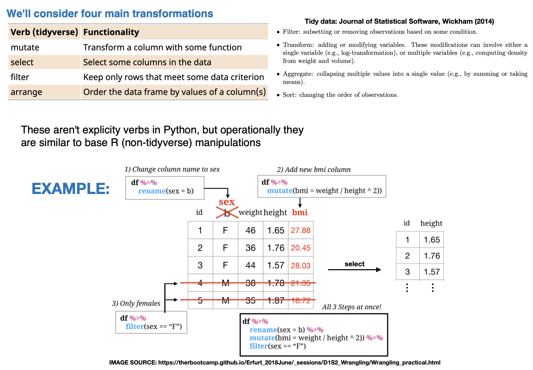
What the tidyverse is

A collection of packages sharing a common design, loaded together with one call.

  • dplyr: data manipulation verbs
  • ggplot2: visualization
  • tidyr: reshaping between wide and long form
  • readr: fast file import
  • tibble, stringr, forcats, purrr: tables, strings, factors, functional tools

Install once, load every session.
Code
# install.packages("tidyverse")   # run once, then comment out
library(tidyverse)

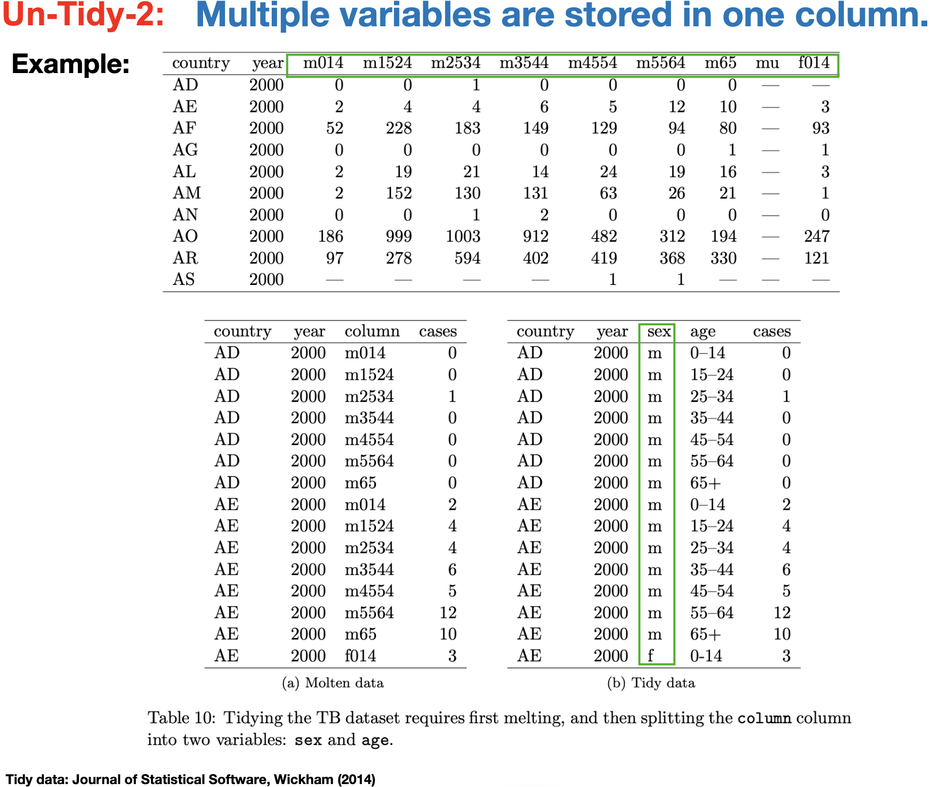
Tidy data

One rule governs everything downstream.

  • Each variable is a column
  • Each observation is a row
  • Each cell is a single value

Data in this shape works directly with every tidyverse function.
Code
mpg          # a tibble shipped with ggplot2: 234 car models
glimpse(mpg) # the tidyverse counterpart to str()
A tibble: 234 × 11
manufacturer model displ year cyl trans drv cty hwy fl class
<chr> <chr> <dbl> <int> <int> <chr> <chr> <int> <int> <chr> <chr>
audi a4 1.8 1999 4 auto(l5) f 18 29 p compact
audi a4 1.8 1999 4 manual(m5) f 21 29 p compact
audi a4 2.0 2008 4 manual(m6) f 20 31 p compact
audi a4 2.0 2008 4 auto(av) f 21 30 p compact
audi a4 2.8 1999 6 auto(l5) f 16 26 p compact
audi a4 2.8 1999 6 manual(m5) f 18 26 p compact
audi a4 3.1 2008 6 auto(av) f 18 27 p compact
audi a4 quattro 1.8 1999 4 manual(m5) 4 18 26 p compact
audi a4 quattro 1.8 1999 4 auto(l5) 4 16 25 p compact
audi a4 quattro 2.0 2008 4 manual(m6) 4 20 28 p compact
audi a4 quattro 2.0 2008 4 auto(s6) 4 19 27 p compact
audi a4 quattro 2.8 1999 6 auto(l5) 4 15 25 p compact
audi a4 quattro 2.8 1999 6 manual(m5) 4 17 25 p compact
audi a4 quattro 3.1 2008 6 auto(s6) 4 17 25 p compact
audi a4 quattro 3.1 2008 6 manual(m6) 4 15 25 p compact
audi a6 quattro 2.8 1999 6 auto(l5) 4 15 24 p midsize
audi a6 quattro 3.1 2008 6 auto(s6) 4 17 25 p midsize
audi a6 quattro 4.2 2008 8 auto(s6) 4 16 23 p midsize
chevrolet c1500 suburban 2wd 5.3 2008 8 auto(l4) r 14 20 r suv
chevrolet c1500 suburban 2wd 5.3 2008 8 auto(l4) r 11 15 e suv
chevrolet c1500 suburban 2wd 5.3 2008 8 auto(l4) r 14 20 r suv
chevrolet c1500 suburban 2wd 5.7 1999 8 auto(l4) r 13 17 r suv
chevrolet c1500 suburban 2wd 6.0 2008 8 auto(l4) r 12 17 r suv
chevrolet corvette 5.7 1999 8 manual(m6) r 16 26 p 2seater
chevrolet corvette 5.7 1999 8 auto(l4) r 15 23 p 2seater
chevrolet corvette 6.2 2008 8 manual(m6) r 16 26 p 2seater
chevrolet corvette 6.2 2008 8 auto(s6) r 15 25 p 2seater
chevrolet corvette 7.0 2008 8 manual(m6) r 15 24 p 2seater
chevrolet k1500 tahoe 4wd 5.3 2008 8 auto(l4) 4 14 19 r suv
chevrolet k1500 tahoe 4wd 5.3 2008 8 auto(l4) 4 11 14 e suv
⋮ ⋮ ⋮ ⋮ ⋮ ⋮ ⋮ ⋮ ⋮ ⋮ ⋮
toyota toyota tacoma 4wd 3.4 1999 6 auto(l4) 4 15 19 r pickup
toyota toyota tacoma 4wd 4.0 2008 6 manual(m6) 4 15 18 r pickup
toyota toyota tacoma 4wd 4.0 2008 6 auto(l5) 4 16 20 r pickup
volkswagen gti 2.0 1999 4 manual(m5) f 21 29 r compact
volkswagen gti 2.0 1999 4 auto(l4) f 19 26 r compact
volkswagen gti 2.0 2008 4 manual(m6) f 21 29 p compact
volkswagen gti 2.0 2008 4 auto(s6) f 22 29 p compact
volkswagen gti 2.8 1999 6 manual(m5) f 17 24 r compact
volkswagen jetta 1.9 1999 4 manual(m5) f 33 44 d compact
volkswagen jetta 2.0 1999 4 manual(m5) f 21 29 r compact
volkswagen jetta 2.0 1999 4 auto(l4) f 19 26 r compact
volkswagen jetta 2.0 2008 4 auto(s6) f 22 29 p compact
volkswagen jetta 2.0 2008 4 manual(m6) f 21 29 p compact
volkswagen jetta 2.5 2008 5 auto(s6) f 21 29 r compact
volkswagen jetta 2.5 2008 5 manual(m5) f 21 29 r compact
volkswagen jetta 2.8 1999 6 auto(l4) f 16 23 r compact
volkswagen jetta 2.8 1999 6 manual(m5) f 17 24 r compact
volkswagen new beetle 1.9 1999 4 manual(m5) f 35 44 d subcompact
volkswagen new beetle 1.9 1999 4 auto(l4) f 29 41 d subcompact
volkswagen new beetle 2.0 1999 4 manual(m5) f 21 29 r subcompact
volkswagen new beetle 2.0 1999 4 auto(l4) f 19 26 r subcompact
volkswagen new beetle 2.5 2008 5 manual(m5) f 20 28 r subcompact
volkswagen new beetle 2.5 2008 5 auto(s6) f 20 29 r subcompact
volkswagen passat 1.8 1999 4 manual(m5) f 21 29 p midsize
volkswagen passat 1.8 1999 4 auto(l5) f 18 29 p midsize
volkswagen passat 2.0 2008 4 auto(s6) f 19 28 p midsize
volkswagen passat 2.0 2008 4 manual(m6) f 21 29 p midsize
volkswagen passat 2.8 1999 6 auto(l5) f 16 26 p midsize
volkswagen passat 2.8 1999 6 manual(m5) f 18 26 p midsize
volkswagen passat 3.6 2008 6 auto(s6) f 17 26 p midsize
Rows: 234
Columns: 11
$ manufacturer <chr> "audi", "audi", "audi", "audi", "audi", "audi", "audi", "…
$ model        <chr> "a4", "a4", "a4", "a4", "a4", "a4", "a4", "a4 quattro", "…
$ displ        <dbl> 1.8, 1.8, 2.0, 2.0, 2.8, 2.8, 3.1, 1.8, 1.8, 2.0, 2.0, 2.…
$ year         <int> 1999, 1999, 2008, 2008, 1999, 1999, 2008, 1999, 1999, 200…
$ cyl          <int> 4, 4, 4, 4, 6, 6, 6, 4, 4, 4, 4, 6, 6, 6, 6, 6, 6, 8, 8, …
$ trans        <chr> "auto(l5)", "manual(m5)", "manual(m6)", "auto(av)", "auto…
$ drv          <chr> "f", "f", "f", "f", "f", "f", "f", "4", "4", "4", "4", "4…
$ cty          <int> 18, 21, 20, 21, 16, 18, 18, 18, 16, 20, 19, 15, 17, 17, 1…
$ hwy          <int> 29, 29, 31, 30, 26, 26, 27, 26, 25, 28, 27, 25, 25, 25, 2…
$ fl           <chr> "p", "p", "p", "p", "p", "p", "p", "p", "p", "p", "p", "p…
$ class        <chr> "compact", "compact", "compact", "compact", "compact", "c…

The pipe

|> passes the result on the left into the first argument of the function on the right.

  • Turns nested calls into a readable top-to-bottom sequence
  • %>% from magrittr is the older form and behaves the same way here
Code
# without the pipe
head(filter(mpg, cyl == 4), 3)

# with the pipe: read it as "take mpg, then filter, then take the head"
mpg |>
  filter(cyl == 4) |>
  head(3)
A tibble: 3 × 11
manufacturer model displ year cyl trans drv cty hwy fl class
<chr> <chr> <dbl> <int> <int> <chr> <chr> <int> <int> <chr> <chr>
audi a4 1.8 1999 4 auto(l5) f 18 29 p compact
audi a4 1.8 1999 4 manual(m5) f 21 29 p compact
audi a4 2.0 2008 4 manual(m6) f 20 31 p compact
A tibble: 3 × 11
manufacturer model displ year cyl trans drv cty hwy fl class
<chr> <chr> <dbl> <int> <int> <chr> <chr> <int> <int> <chr> <chr>
audi a4 1.8 1999 4 auto(l5) f 18 29 p compact
audi a4 1.8 1999 4 manual(m5) f 21 29 p compact
audi a4 2.0 2008 4 manual(m6) f 20 31 p compact

The core dplyr verbs

Five functions cover most day-to-day data manipulation.

  • filter(): keep rows matching a condition
  • select(): keep columns
  • mutate(): add or modify columns
  • arrange(): sort rows, desc() for descending
  • summarize(): collapse many rows into one
Code
mpg |>
  filter(class == "compact") |>
  select(manufacturer, model, displ, hwy) |>
  mutate(km_per_liter = hwy * 0.425) |>
  arrange(desc(hwy)) |>
  head(5)
A tibble: 5 × 5
manufacturer model displ hwy km_per_liter
<chr> <chr> <dbl> <int> <dbl>
volkswagen jetta 1.9 44 18.700
toyota corolla 1.8 37 15.725
toyota corolla 1.8 35 14.875
toyota corolla 1.8 33 14.025

Group and summarize

group_by() splits the data, summarize() collapses each group, and the result is one row per group.

  • This single pattern replaces most of what pivot tables do
  • n() counts rows within the current group
Code
mpg |>
  group_by(class) |>
  summarize(
    n        = n(),
    mean_hwy = mean(hwy),
    mean_cty = mean(cty)
  ) |>
  arrange(desc(mean_hwy))
A tibble: 7 × 4
class n mean_hwy mean_cty
<chr> <int> <dbl> <dbl>
compact 47 28.29787 20.12766
subcompact 35 28.14286 20.37143
midsize 41 27.29268 18.75610
2seater 5 24.80000 15.40000
minivan 11 22.36364 15.81818
suv 62 18.12903 13.50000
pickup 33 16.87879 13.00000

Reshaping with tidyr

  • pivot_longer() turns wide data into long data, which is what plotting functions expect
  • pivot_wider() reverses it
Code
long <- mpg |>
  select(model, cty, hwy) |>
  pivot_longer(cols = c(cty, hwy),
               names_to  = "measure",
               values_to = "mpg")

head(long)
A tibble: 6 × 3
model measure mpg
<chr> <chr> <int>
a4 cty 18
a4 hwy 29
a4 cty 21
a4 hwy 29
a4 cty 20
a4 hwy 31