Optimizing a linear objective under linear constraints
Math review
Linear equations; Quick detour
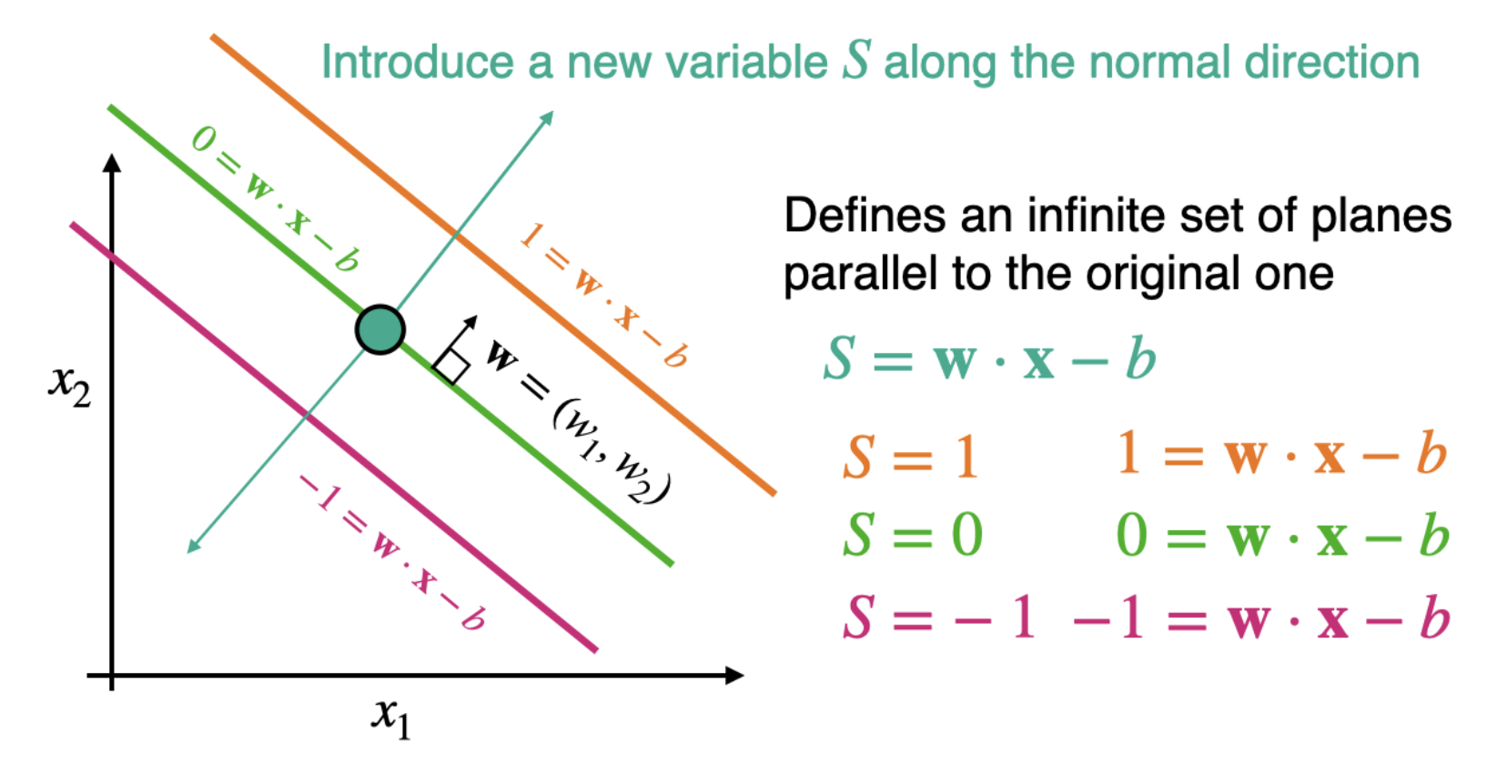
Recall: Equations of planes in higher dimensions
Equation of a Plane in 2D: - A line in 2D can be written as:
\[
a x_1+b x_2+c=0
\]
\(a, b\) define the direction of the line; \(c\) is the offset.
Equation of a Plane in 3D:
A plane in 3D is given by:
\[
a x_1+b x_2+c x_3+d=0
\]
The normal vector \((a, b, c)\) defines the plane’s orientation.
Equation of a Hyperplane in N-D Space:
General form in \(N\)-dimensional space:
\[
w_1 x_1+w_2 x_2+\cdots+w_N x_N+b=0
\]
\({ }^{-} w\) is the normal vector, \(b\) is the bias term. - Separates \(N\)-dimensional space into two half-spaces.
Normal vector
The equation of a plane in 3D can be written using the normal vector \(\vec{n}=\langle a, b, c\rangle\) and a point on the plane \(P_0=\left(x_0, y_0, z_0\right)\) as:
where: - \(a, b, c\) are the components of the normal vector \(\vec{n}\), - \(d=a x_0+b y_0+c z_0\) is a constant determined by the point on the plane.
Finally, using dot product notation, the equation of a plane in 3D can be written as:
\(\vec{n} \cdot (\vec{r} - \vec{r}_0) = 0\)
Where:
\(\vec{n} = \langle a, b, c \rangle\) is the normal vector to the plane,
\(\vec{r} = \langle x, y, z \rangle\) is a position vector to any point on the plane,
\(\vec{r}_0 = \langle x_0, y_0, z_0 \rangle\) is the position vector of a known point on the plane.
This form expresses that the vector from \(\vec{r}_0\) to \(\vec{r}\) is orthogonal to the normal vector \(\vec{n}\), hence lies in the plane.
Example
Overiew of linear programming
Optimization: Big picture
A huge range of problems in data science, economics, and engineering reduce to one question:
what is the best choice among many allowed options?
Optimization means choosing values for some variables to make an objective as large or as small as possible, while obeying a set of rules
Every optimization problem has three ingredients:
Decision variables: the quantities we get to control
Objective function: the single number we want to maximize or minimize
Constraints: the rules that limit which choices are allowed
Linear programming is the simplest and most widely used member of this family, so it is the natural place to start
General constrained optimization problem
An constrained optimization problem involves finding the values of decision variables that minimize (or maximize) an objective function, subject to a set of constraints:
Feasible solution: any assignment of the variables that satisfies all constraints
Feasible region: the set of every feasible solution
Optimal solution: a feasible solution that achieves the best objective value
Infeasible problem: the constraints contradict each other, so no solution exists
Unbounded problem: the objective can be improved forever with no ceiling (for example, maximizing profit with no resource limits)
Well posed LPs that we solve in practice are feasible and bounded, giving a finite best answer
The Geometry of LP
The Feasible Region Is a Polytope
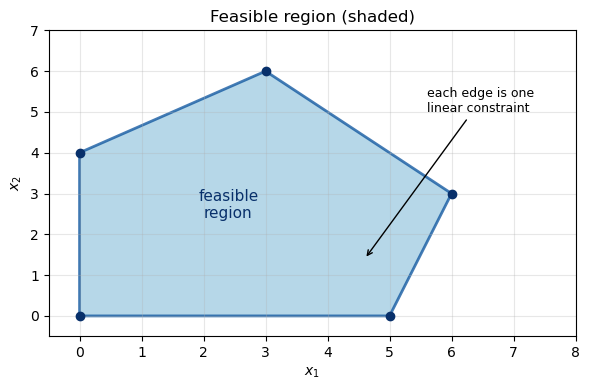
Each linear constraint splits space into an allowed side and a forbidden side, called a half-space
The feasible region is the intersection of all these half-spaces
The result is a convex polytope: a flat-sided shape with no dents or holes
convex means the straight line between any two feasible points stays entirely inside the region
This shape is the stage on which the whole problem plays out
Figure 1: A feasible region is the intersection of half-spaces, forming a convex polytope.
The Fundamental Theorem of LP
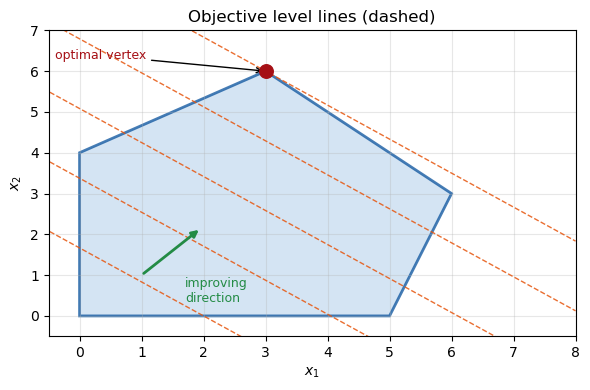
The objective \(Z = \mathbf{c}^\top \mathbf{x}\) has straight, parallel level lines: sets of points that all give the same value of \(Z\)
Improving the objective means sliding those level lines as far as possible in one direction
Key insight: the last point of contact with the feasible region is always a corner (vertex)
Fundamental theorem of LP: if an optimal solution exists, at least one optimal solution lies at a vertex of the feasible region
we never have to search the interior
we only need to inspect the finite set of corners
Figure 2: Sliding the objective level lines: the optimum lands on a corner.
Worked Example
The Furniture Workshop
A small workshop builds chairs and tables and wants to maximize profit
Decision variables:
\(x_1\) = number of chairs, \(x_2\) = number of tables
Objective (profit in dollars):
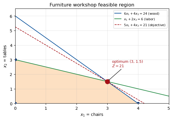
\(\max \; Z = 5x_1 + 4x_2\)
Constraints (two limited resources):
wood: \(6x_1 + 4x_2 \le 24\)
labor: \(x_1 + 2x_2 \le 6\)
nonnegativity: \(x_1 \ge 0, \; x_2 \ge 0\)
Goal: find the mix of chairs and tables that earns the most, without running out of wood or labor
Checking the Corners
By the fundamental theorem, the optimum sits at a vertex, so we just evaluate \(Z = 5x_1 + 4x_2\) at each corner
Corner \((x_1, x_2)\)
Binding limits
\(Z = 5x_1 + 4x_2\)
\((0, 0)\)
origin
\(0\)
\((4, 0)\)
wood
\(20\)
\((0, 3)\)
labor
\(12\)
\((3, 1.5)\)
wood and labor
\(\mathbf{21}\)
The best corner is \((3, 1.5)\), where both resources are fully used
Answer: build \(3\) chairs and \(1.5\) tables for a profit of \(Z = 21\)
Figure 3: The workshop LP: feasible region, corner points, and the optimum.
Numerical Solver methods
The Simplex Method
Checking every corner by hand works for two variables, but the number of corners explodes as problems grow
The simplex method (Dantzig, 1947) is smarter:
start at one corner of the feasible region
repeatedly step to an adjacent corner that improves the objective
stop when no neighboring corner is better, which guarantees the optimum
Intuition: walk along the edges of the polytope, always uphill, until you reach the peak
In practice it is very fast and remains a workhorse decades later
Interior Point Methods and Duality
Interior point methods take a different route:
instead of hugging the edges, they cut through the middle of the region and converge on the optimal corner
they scale extremely well to very large problems
Duality is a deep idea worth knowing at a glance:
every LP (the primal) has a partner problem called the dual
the dual’s variables act as shadow prices: the value of one more unit of each scarce resource
primal and dual optimal objective values are equal, which gives a built-in optimality check
Modern solvers pick the method for you, so you mostly just describe the problem
LP in Data Science
Where You Will Meet LP
Resource allocation: budgets, staffing, production mixes (our workshop, at scale)
Transportation and logistics: move goods from warehouses to stores at least cost
Network flow: routing traffic, data, or supply through a network
L1 regression and LASSO-style fits: several robust regression objectives reduce to LPs
Support vector machines: the linear, hinge-loss variant is a linear (or quadratic) program
Preprocessing and fairness: optimal matching, assignment, and reweighting problems
Takeaway: LP is a reusable engine. Learn to spot the pattern of “linear objective, linear limits” and you can hand the problem to a solver
A Note on Assumptions
LP assumes three things that are worth remembering:
linearity: objective and constraints are linear (no curves or interactions)
divisibility: fractional answers are allowed, like \(1.5\) tables
certainty: the coefficients are known and fixed
If variables must be whole numbers, you need integer programming, which is a harder, related problem
If relationships curve, you move to nonlinear or convex optimization
LP is the foundation these richer methods build on
Solving LP in Python
Tooling
Two common, easy to install options:
SciPy (scipy.optimize.linprog): already in the standard scientific stack, great for a first solve
PuLP: a friendly modeling language that reads almost like the math, good for larger models
We will use SciPy here for the “hello world” solve
Convention: SciPy minimizes and expects constraints as \(A\mathbf{x} \le \mathbf{b}\)
to maximize, we minimize the negative of the objective
We will keep the problem in a structured dictionary so it is easy to log, swap, or feed into an automated search over scenarios
Defining the Problem
Separating the problem definition from the solve is a best practice
The config below is data, not logic, so it could be loaded from a file or generated in a loop
Note the clean fields: an objective vector, a list of constraints, and variable bounds
Code
import numpy as npfrom scipy.optimize import linprog# Problem kept as a structured config: easy to log, swap, or sweep.LP_PROBLEM = {"sense": "maximize", # "maximize" or "minimize""variables": ["chairs", "tables"], # decision variable names"objective": [5.0, 4.0], # profit per unit"constraints": [# each row: name, coefficients, comparison operator, right-hand side {"name": "wood", "coeffs": [6.0, 4.0], "op": "<=", "rhs": 24.0}, {"name": "labor", "coeffs": [1.0, 2.0], "op": "<=", "rhs": 6.0}, ],"bounds": [(0, None), (0, None)], # nonnegativity by default}
Solving and Interpreting
A small translator turns the config into the arguments SciPy expects
method="highs" selects a modern, reliable solver (SciPy’s current default)
We flip the sign back at the end to report the true maximized profit
Code
def build_linprog_args(problem):"Translate the config dict into SciPy linprog arguments." sign =-1.0if problem["sense"] =="maximize"else1.0 c = [sign * ci for ci in problem["objective"]] A_ub, b_ub = [], []for con in problem["constraints"]: coeffs, op, rhs = con["coeffs"], con["op"], con["rhs"]if op =="<=": A_ub.append(coeffs) b_ub.append(rhs)elif op ==">=": # flip to <= form A_ub.append([-a for a in coeffs]) b_ub.append(-rhs)else:raiseValueError("Split equalities into two inequalities.")return c, A_ub, b_ub, problem["bounds"]c, A_ub, b_ub, bounds = build_linprog_args(LP_PROBLEM)result = linprog(c=c, A_ub=A_ub, b_ub=b_ub, bounds=bounds, method="highs")opt_value =-result.fun if LP_PROBLEM["sense"] =="maximize"else result.funprint("Status:", result.message)for name, val inzip(LP_PROBLEM["variables"], result.x):print(f" {name:>7} = {val:5.2f}")print(f" optimal profit = {opt_value:5.2f}")