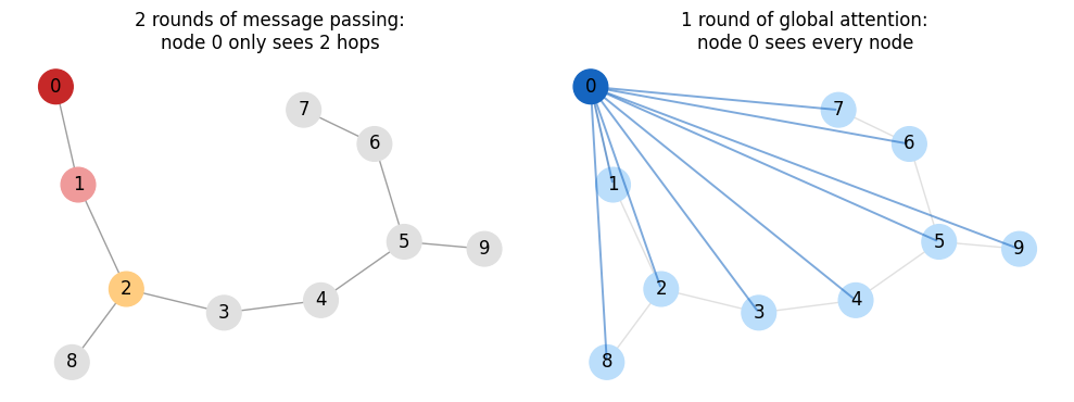
It combines them with a permutation invariant operation (sum, mean, or max), so the answer does not depend on the arbitrary order the neighbors were listed in
It mixes that summary with its own current state to produce a new state
The consequence: after \(L\) layers, a node’s representation depends only on nodes within \(L\) hops. Information travels one edge per layer.
Core Limitations of Message Passing in GNNs
Limited receptive field: Information only propagates one hop per layer; influencing nodes 10 hops apart requires ≥10 layers. Most GNNs use just 2–5 layers due to training difficulties.
Oversquashing: Large neighborhoods get compressed into a fixed-size vector—critical information can be lost, especially across bottleneck edges.
Oversmoothing: Repeated aggregation makes node representations alike; too many layers, and all nodes become indistinguishable.
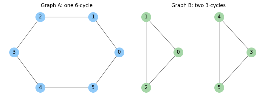
Limited expressivity: Message passing has an upper limit on its power. If two graphs yield identical node label multisets, a standard GNN cannot tell them apart.
Example: Where Message Passing Fails
Setup
Two graphs: each with 6 nodes, 6 edges; every node has exactly 2 neighbors
All nodes initialized with the same feature (e.g., \(1\))
Message Passing Outcome
At every round, nodes aggregate neighbors’ identical features, producing identical results
Repeated rounds yield byte-for-byte identical node embeddings across both graphs
Key Points
Humans easily spot the difference (connected vs. disconnected)
Distinction is global (e.g., connectivity), but message passing is local
We’ll train a graph transformer to solve this at the end of the lecture
The Naive Graph Transformer
The Key Idea
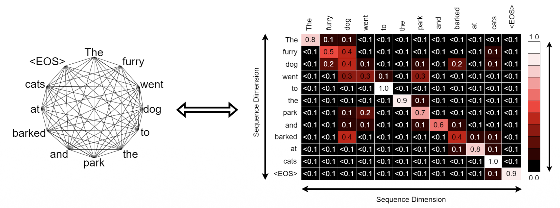
The transformer is a GNN on a fully connected graph
Each element attends to all others—identical to message passing on a complete graph
Attention weights \(\alpha_{ij}\) are learned, data-dependent edge weights
Aggregation is a permutation-invariant weighted sum, just like GNN aggregation
Implications
The receptive field covers the entire graph in a single layer—no bottleneck oversquashing
Any two nodes can interact directly, regardless of distance
However, without edge information, a set of nodes alone destroys structure; the model cannot infer graph edges (e.g., molecule bonds or word order) without explicit encodings
Self Attention
Stack the \(N\) node feature vectors as rows of a matrix \(H \in \mathbb{R}^{N \times d}\). Learn three weight matrices and project:
Key\(k_j\): what node \(j\) advertises about itself
Value\(v_j\): what node \(j\) actually hands over if attended to
Softmax: turns a row of arbitrary real numbers into positive weights that sum to 1, via \(\text{softmax}(x)_i = e^{x_i} / \sum_j e^{x_j}\)
\(\sqrt{d_k}\): a scaling constant that keeps dot products from growing with dimension and saturating the softmax
Step by step, for a single node \(i\)
Compute a compatibility score with every node \(j\): \(\ s_{ij} = \dfrac{q_i \cdot k_j}{\sqrt{d_k}}\)
The dot product is large when two vectors point in similar directions, so this is a learned similarity
Normalize the scores across \(j\) with a softmax to get weights \(\alpha_{ij} \ge 0\) with \(\sum_j \alpha_{ij} = 1\)
Output a weighted average of the values: \(\ z_i = \sum_j \alpha_{ij} v_j\)
Multi head attention simply does this \(h\) times in parallel with separate weight matrices and concatenates the results, so different heads can specialize (one on nearby nodes, one on a particular substructure, and so on).
Something is missing …
Structure. A plain transformer over nodes is permutation equivariant in the wrong way: it treats the graph as an unordered set.
Two graphs a naive transformer cannot distinguish
A benzene ring and six carbon atoms floating in a vacuum have the same node set
Only the edges differ, and the edges are the part we threw away
The design problem
Reinject the structure so attention becomes graph aware
Do it without destroying the property we wanted, namely direct all pairs communication
Keep the whole thing permutation equivariant: relabeling the nodes should permute the outputs in the same way and nothing else
Toy Example Calculation
This is just a toy example to demonstrate the idea we use a very simple structural embedding that is NOT realistic!
The Setup
A graph with 3 nodes:\(A - B - C\), a simple path. Node \(B\) is in the middle.
Raw features (imagine two measured properties per node), with \(d = 2\):
Nodes \(A\) and \(C\) share the same degree vector.
Why:
Raw features alone provide no position information—the encoding signals that \(B\) is a hub.
Step 2: Queries, Keys, Values
Because we chose identity weight matrices,
\[q_i = k_i = v_i = h_i\]
so
node
\(q_i\)
\(k_i\)
\(v_i\)
A
\([1.5, 0]\)
\([1.5, 0]\)
\([1.5, 0]\)
B
\([0, 1.5]\)
\([0, 1.5]\)
\([0, 1.5]\)
C
\([1.5, 1]\)
\([1.5, 1]\)
\([1.5, 1]\)
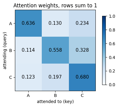
Consider node \(A\) as the query for the next few slides. We will compute how much \(A\) attends to each of the three nodes, then what new vector \(A\) ends up with.
Step 3: Raw Similarity Scores
With \(d_k = 2\) we divide by \(\sqrt{2} \approx 1.414\):
\(q_A \cdot k_A = (1.5)(1.5) + (0)(0) = 2.25\), so the score is \(2.25 / 1.414 = 1.591\)
\(q_A \cdot k_B = (1.5)(0) + (0)(1.5) = 0\), so the score is \(0\)
\(q_A \cdot k_C = (1.5)(1.5) + (0)(1) = 2.25\), so the score is \(1.591\)
Notice the problem. Based on features alone, \(A\) finds itself and \(C\) equally compatible, even though \(C\) is two hops away and \(B\) is its only actual neighbor. Content similarity has no idea what the graph looks like. (because so far we used a toy structural embedding!)
Step 4: Add the Distance Bias (more structural encoding)
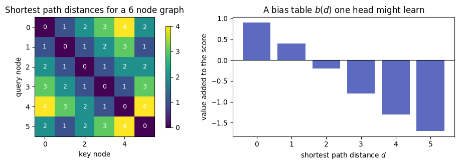
Shortest path distances from \(A\) are \(\text{dist}(A,A) = 0\), \(\text{dist}(A,B) = 1\), \(\text{dist}(A,C) = 2\). Suppose the learned bias table currently holds
\[b(0) = 0, \qquad b(1) = 0, \qquad b(2) = -1\]
Adding \(b(\text{dist})\) to each raw score gives the final scores for row \(A\):
These are positive and sum to \(1\), so they are a genuine weighted average. Repeating the same three steps with \(B\) and \(C\) as the query fills in the rest of the matrix.
Step 6: Weighted Sum of Values
The new state of node \(A\) is \(z_A = \sum_j \alpha_{Aj} v_j\):
So \(z_A = [1.305, 0.429]\), and the same procedure gives \(z_B = [0.663, 1.165]\) and \(z_C = [1.204, 0.975]\).
The headline: node \(A\) pulled 23 percent of its new state directly from node \(C\), which it is not connected to. A one layer message passing GNN would give \(C\) a weight of exactly zero.
Step 7: Readout, Prediction, and Loss
Mean pooling over the three nodes gives a single graph vector:
That is one complete forward pass, from raw node features to a scalar loss.
Step 8: What Backpropagation Updates
The gradient starts at \(\dfrac{\partial \mathcal{L}}{\partial \hat{y}} = 2(\hat{y} - y) = 1.828\) and flows backward through every step we just did. The learnable pieces are
The readout weights \(w\)
The projection matrices \(W_Q\), \(W_K\), \(W_V\) (which we pinned to the identity, but normally are free)
The degree encoding table\(c_{\text{deg}}\), so the model learns what a hub node should look like
The distance bias table\(b(d)\), so the model learns how far attention should reach
This is the part worth remembering. The structural priors are not fixed hyperparameters that you tune by hand. They are parameters, and the model discovers from data how much graph distance should matter for your task.
Structural encoding
Looking closer at making Attention Graph Aware
Three possible places to inject structure
Node features (positional/structural encodings)
Add per-node vectors capturing graph position/structure to input features
Ex: Laplacian eigenvectors, random walk probabilities, node degree
Attention scores (structural bias)
Modify \(s_{ij}\) with learned terms reflecting \(i,j\) relationships
Ex: shortest path, edge presence/type
Model architecture (hybrid layers)
Combine message passing and attention blocks in each layer
Local branch: structure; global branch: long-range interactions
Most modern models use several of these together.
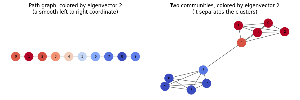
Phonons as Laplacian Eigenvectors
1D harmonic chain (ring of \(N\) atoms)
Nearest-neighbor springs \(K\), masses \(m\)
Equation of motion: \(m\,\ddot{x}_n = K\,(x_{n+1} + x_{n-1} - 2x_n)\)
In matrix form: \(m\,\ddot{\mathbf{x}} = -K\,L\,\mathbf{x}\), where \(L = D - A\) is the graph Laplacian of the ring
Stack first \(k\) eigenvectors: \(p_i = [\,u_1(i), \ldots, u_k(i)\,]\) is a positional encoding
Same object physics calls a phonon basis, graph ML calls a Laplacian PE
Key Idea
Laplacian eigenvector spectrum:
Small \(\lambda\): long wavelength \(\rightarrow\) smooth, global variation across the graph (coarse coordinates).
Large \(\lambda\): short wavelength \(\rightarrow\) rapid sign-flipping between adjacent nodes; captures fine local structure but not restricted to a region—still fully supported on the whole graph.
“Local” = rapid change across edges, not limited support:
High-frequency eigenvectors oscillate on the length scale of a single edge but extend globally.
True spatial localization is due to disorder, not just large eigenvalue.
Phonon analogy:
Small \(q\): atoms move almost in unison (acoustic modes).
Large \(q \to \pi\): adjacent atoms move in opposition (zone-boundary modes).
Same operator, same global vs local distinction in eigenmodes.
Option-1: Adding Laplacian PEs to Node Features
Per-node encoding vector
Stack the first \(k\) nontrivial eigenvectors columnwise, read off row \(i\)
Shapes: each \(u_j \in \mathbb{R}^{n}\) (one value per node), stacked into \(U = [\,u_1 \mid u_2 \mid \cdots \mid u_k\,] \in \mathbb{R}^{n \times k}\), so row \(i\) gives \(p_i \in \mathbb{R}^{k}\)
Needs a learned projection since \(k \neq d\) in general
Sign ambiguity
\(u\) and \(-u\) are both valid eigenvectors, so \(p_i\) has no canonical sign
Fix: random sign flips \(p_i \rightarrow S p_i\) per epoch, or sign-invariant encoders (SignNet)
Do Laplacian PEs Break Inductive Learning?
Two “size” notions: - Per-node PE dimension \(k\): fixed, graph-independent—enables any-graph input - Each eigenvector \(u_j \in \mathbb{R}^n\): global, depends on all \(n\) nodes
Why Laplacian PEs are transductive - Eigenvector \(j\) has no consistent meaning or alignment across graphs - Degenerate eigenvalues: freedom in basis rotation and sign; unstable under small graph changes - Adding/removing nodes shifts all encodings unpredictably
Key transformer difference - Sinusoidal PE: strictly index-based, transferable across samples - Laplacian PE: structure-dependent, unique per graph
Toward inductive transfer - Retrain for sign/basis invariance (e.g., SignNet, BasisNet) per graph - Involves costly eigendecomposition per instance - Prefer local node encodings (random-walk PEs, shortest-path distances) for better transfer and efficiency
Random Walk Encodings: Simple & Effective
Transition matrix: \(M = D^{-1} A\), with \(M_{ij}\) as probability of stepping \(i \to j\)
Encode node \(i\) by vector of return probabilities: \(\big[(M^1)_{ii}, (M^2)_{ii}, \ldots, (M^k)_{ii}\big]\)
Captures: likelihood of returning to origin after \(t\) steps; useful for detecting triangles, cycles, density patterns
No sign problem, often performs comparably
Option-2: Distance Bias in the Scores
Modify the attention score with an additive term that depends on graph structure:
\(\text{dist}(i,j)\) is the shortest path distance, the minimum number of edges to walk from \(i\) to \(j\)
\(b(\cdot)\) is a small lookup table of learnable scalars, one per distance value, and one extra entry for “no path exists”
Because the bias is added before the softmax, it acts as a soft prior: the model can learn to favor close nodes without being forbidden from attending far away
Each attention head gets its own table, so one head can specialize in neighbors while another looks globally
This is the core trick of Graphormer, which won the 2021 Open Graph Benchmark large scale challenge on molecular property prediction.
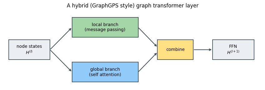
Option 3: Keep a Local Branch
Two ways nodes gather information - Message passing: each node receives info only from direct neighbors - Attention: each node can access all others at once
Key intuitions - Message passing: like talking with people in your room—detailed, grounded, but slow for distant nodes - Attention: like a group video call—immediate global reach, but loses local structure
Why combine both in one layer? - Local branch preserves actual graph connections - Global branch enables instant communication with distant but relevant nodes - Each layer merges local and global info, updating nodes with both nearby and far context
Benefits of hybrid approach - Pure message passing: slow, bottlenecked distant communication; deep stacks oversmooth node features - Pure attention: immediate reach but ignores graph structure unless positional info added - Hybrid: combines local structure with global reach, mitigating both issues
The Full Graph Transformer Layer
A single layer, in the order the operations actually run:
Normalize:\(\tilde{H} = \text{LayerNorm}(H)\), which rescales each node vector to zero mean and unit variance for training stability
Attend:\(A = \text{MultiHeadAttention}(\tilde{H})\) with the structural bias added to the scores
Residual:\(H' = H + A\), so the layer learns a correction rather than a replacement, which keeps gradients flowing in deep stacks
Feed forward:\(H'' = H' + \text{MLP}(\text{LayerNorm}(H'))\), a two layer network applied independently to each node, usually expanding the width by 2 to 4 times and back
Then, for a graph level prediction - Readout: Pool node vectors into a single graph vector (via mean/sum pooling or a dedicated virtual node). - Virtual node: Add a node connected to all others. At each layer: - Learns global features during message passing. - Serves as a communication shortcut: any node pair can connect in two hops, improving long-range info flow and reducing bottlenecks. - Head: Final graph vector is fed to a small MLP for output (logits or regression).
Scaling Strategies
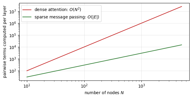
The problem: the attention matrix has \(N^2\) entries. A molecule with 50 atoms is trivial. A social network with 100 million nodes is impossible.
Common escapes
Small graphs only. Molecules, small circuits, and program graphs mostly have tens to hundreds of nodes, which is where graph transformers are most used today
Sparse or windowed attention. Attend only to a sampled subset, or only within some hop radius, plus a few random long range links
Linear attention. Approximate the softmax with kernel tricks to get \(O(N)\) cost, at some loss of fidelity
Virtual nodes. Add one extra node connected to everything. Every pair can now communicate in two hops at \(O(N)\) cost. Cheap, and surprisingly effective
Hybrid layers. GraphGPS runs sparse message passing and global attention in parallel, so you pay the quadratic cost only in the global branch, which can then be a linear approximation
When to Use Graph Transformers
Best for: - Small to medium graphs (≤ few thousand nodes) - Tasks needing global structure: molecular shape, long-range dependencies, overall connectivity - Large datasets (transformers require more data due to weaker inductive bias) - GNN accuracy has plateaued; deeper GNNs degrade performance
Poor fit for: - Very large graphs (quadratic attention is prohibitive) - Small datasets, where GNN locality acts as a helpful prior - Problems that are purely local (e.g., typical node classification on homophilous networks)
Summary:
A strong GNN baseline usually suffices; use graph transformers when true global reasoning is essential.
Single fixed graph, transductive node classification, homophilous graphs where neighbors share labels; strong simple baseline
Simple, few parameters, fast; smooths features well on homophilous graphs; solid default baseline
Transductive by default (uses full normalized adjacency); all neighbors weighted equally; oversmooths with depth; struggles on heterophilous graphs; needs whole graph in memory
GAT: attention-weighted aggregation Examples: GAT (Veličković), GATv2 (fixes static-attention flaw), attention variants in molecular models
When neighbors should count unequally and you want learned, interpretable edge weights; heterophily; graphs where a few neighbors dominate
Learns per-edge importance; multi-head stabilizes and enriches; attention gives some interpretability; no eigendecomposition needed
More parameters and compute than GCN; original GAT has “static attention” (GATv2 addresses it); still local message passing, so oversmoothing and limited receptive field remain
Inductive settings, large/streaming graphs, unseen nodes at test time, minibatch training that can’t fit the full graph
Genuinely inductive (learns aggregator functions, not per-node embeddings); neighbor sampling scales to billions of edges; multiple aggregators (mean/LSTM/pool)
Sampling adds variance and misses some neighbors; fixed sample size caps receptive field; aggregator choice matters; still local, so long-range dependencies are hard
Graph Transformers: global self-attention over nodes + structural/positional encodings Examples: Graphormer, SAN, GraphGPS (GPS), TokenGT, Exphormer
Every node attends to every node in one layer (no oversmoothing/bottleneck); encodes structure via PEs (e.g., Laplacian) and edge biases; state-of-the-art on many graph-level benchmarks
\(O(n^2)\) attention limits graph size (linear-attention variants like Exphormer mitigate); relies on positional encodings that are often transductive/unstable (the Laplacian-PE issue from earlier); data-hungry
Recommended Reading
Dwivedi and Bresson (2020), A Generalization of Transformer Networks to Graphs. The first clean graph transformer with Laplacian positional encodings
Ying et al. (2021), Do Transformers Really Perform Bad for Graph Representation? Introduces Graphormer, including the centrality and shortest path bias terms used above
Kreuzer et al. (2021), Rethinking Graph Transformers with Spectral Attention
Rampasek et al. (2022), Recipe for a General, Powerful, Scalable Graph Transformer. The GraphGPS hybrid framework
Alon and Yahav (2021), On the Bottleneck of Graph Neural Networks and its Practical Implications. The clearest treatment of oversquashing
Xu et al. (2019), How Powerful are Graph Neural Networks? The Weisfeiler-Lehman expressivity result
Summary
Message passing is local by construction, which causes limited receptive fields, oversquashing, oversmoothing, and a hard ceiling on expressivity at the 1-Weisfeiler-Lehman test
A transformer is a GNN on a complete graph, so it gets global communication in one layer but starts out blind to the actual edges
A graph transformer reinjects structure in three complementary ways: positional encodings on nodes, structural bias on attention scores, and hybrid local plus global layers
Laplacian eigenvectors are the graph version of sinusoidal positions, and random walk encodings are a convenient alternative
The structural priors are learned, not fixed. The bias table \(b(d)\) lets the model decide for itself how far attention should reach
Cost is the main constraint. Dense attention is \(O(N^2)\), which is why graph transformers dominate on molecules and struggle on web scale networks
A tuned GNN is still a strong baseline. Reach for a transformer when the task genuinely needs global reasoning
Code Demo:
The Task
Binary classification of featureless graphs
Class 0: a single cycle of \(n\) nodes
Class 1: two disjoint cycles whose sizes add to \(n\)
\(n\) varies between 10 and 14, and node labels are randomly permuted
Why this task
Every node in both classes has degree exactly 2, and there are no node features to help
This is the counterexample from earlier, so a standard message passing GNN is at chance, near 50 percent, no matter how long you train it
The distinguishing information is purely global: is this one component or two?
What we will build: a compact graph transformer with Laplacian positional encodings, per head shortest path distance bias, pre-norm residual blocks, masked pooling, and a hyperparameter dictionary ready to drop into a search.
Setup and Hyperparameters
Note on the config dictionary: every knob lives in one place, so this object can be handed directly to a grid search, Optuna, or Ray Tune without touching the model code.
Code
import mathimport numpy as npimport networkx as nximport torchimport torch.nn as nnimport torch.nn.functional as FCONFIG = {# data"seed": 0,"n_graphs": 1000,"min_nodes": 10,"max_nodes": 14,"train_frac": 0.8,# structural features"pe_dim": 6, # number of Laplacian eigenvectors used per node"max_spd": 6, # distances are clipped here; one extra bucket means unreachable# model"d_model": 64,"n_heads": 4,"n_layers": 3,"ffn_mult": 2,"dropout": 0.1,# optimization"lr": 1e-3,"weight_decay": 1e-2,"batch_size": 32,"epochs": 15,"grad_clip": 1.0,}torch.manual_seed(CONFIG["seed"])rng = np.random.default_rng(CONFIG["seed"])device = torch.device("cuda"if torch.cuda.is_available() else"cpu")print("device:", device)
device: cpu
Generating the Dataset
Code
def make_graph(label, rng, cfg):"""Label 0: one cycle. Label 1: two disjoint cycles with the same total size.""" n =int(rng.integers(cfg["min_nodes"], cfg["max_nodes"] +1))if label ==0: G = nx.cycle_graph(n)else: a =int(rng.integers(3, n -2)) # both pieces must be at least a triangle G = nx.disjoint_union(nx.cycle_graph(a), nx.cycle_graph(n - a)) perm = rng.permutation(n) # node order must not leak the labelreturn nx.relabel_nodes(G, {i: int(perm[i]) for i inrange(n)})# Sanity check: the two classes are indistinguishable to a degree based modelseqs =set()for label in (0, 1): G = make_graph(label, np.random.default_rng(1), CONFIG) seqs.add(tuple(sorted(d for _, d in G.degree())))print("distinct degree sequences across the two classes:", len(seqs))
distinct degree sequences across the two classes: 1
Structural Features
Two tensors per graph
pe: the Laplacian positional encoding, one vector of length pe_dim per node
spd: an integer matrix of bucketed shortest path distances, used to index the learned bias table
The extra bucket at index max_spd + 1 encodes “no path exists”, which is precisely the signal that separates our two classes.
Code
def laplacian_pe(G, k):"""First k nontrivial eigenvectors of the symmetric normalized Laplacian.""" nodes =sorted(G.nodes()) A = nx.to_numpy_array(G, nodelist=nodes) deg = A.sum(axis=1) dinv = np.where(deg >0, 1.0/ np.sqrt(np.maximum(deg, 1e-12)), 0.0) L = np.eye(len(nodes)) - (dinv[:, None] * A * dinv[None, :]) _, evecs = np.linalg.eigh(L) # eigh returns ascending eigenvalues pe = evecs[:, 1:k +1] # skip the trivial constant eigenvectorif pe.shape[1] < k: # pad if the graph is smaller than k + 1 pe = np.pad(pe, ((0, 0), (0, k - pe.shape[1])))return pe.astype(np.float32)def spd_buckets(G, max_spd):"""Pairwise shortest path distances, clipped, with a dedicated unreachable bucket.""" n = G.number_of_nodes() D = np.full((n, n), max_spd +1, dtype=np.int64)for i, dists in nx.all_pairs_shortest_path_length(G):for j, d in dists.items(): D[i, j] =min(d, max_spd)return Ddef build_dataset(cfg, rng): items = []for i inrange(cfg["n_graphs"]): label = i %2# perfectly balanced classes G = make_graph(label, rng, cfg) items.append({"n": G.number_of_nodes(),"pe": laplacian_pe(G, cfg["pe_dim"]),"spd": spd_buckets(G, cfg["max_spd"]),"y": label, })return itemsdata = build_dataset(CONFIG, rng)rng.shuffle(data)cut =int(CONFIG["train_frac"] *len(data))train_set, test_set = data[:cut], data[cut:]print(f"train graphs: {len(train_set)} test graphs: {len(test_set)}")
train graphs: 800 test graphs: 200
Batching Variable Sized Graphs
Graphs in a batch have different node counts, so we pad to max_nodes and carry a boolean mask. The mask does two jobs: it blocks attention to padded slots and it keeps padding out of the pooled graph vector.
Code
def collate(batch, cfg): B, N =len(batch), cfg["max_nodes"] pe = torch.zeros(B, N, cfg["pe_dim"]) spd = torch.full((B, N, N), cfg["max_spd"] +1, dtype=torch.long) mask = torch.zeros(B, N, dtype=torch.bool) y = torch.zeros(B, dtype=torch.long)for b, item inenumerate(batch): n = item["n"] pe[b, :n] = torch.from_numpy(item["pe"]) spd[b, :n, :n] = torch.from_numpy(item["spd"]) mask[b, :n] =True y[b] = item["y"]return pe.to(device), spd.to(device), mask.to(device), y.to(device)def batches(dataset, cfg, shuffle, rng): idx = np.arange(len(dataset))if shuffle: rng.shuffle(idx)for start inrange(0, len(idx), cfg["batch_size"]):yield collate([dataset[i] for i in idx[start:start + cfg["batch_size"]]], cfg)def flip_eigenvector_signs(pe):"""Sign of an eigenvector is arbitrary, so randomize it as a training augmentation.""" signs = torch.randint(0, 2, (pe.shape[0], 1, pe.shape[2]), device=pe.device) *2-1return pe * signs
The Attention Module
This is the one piece that differs from a standard transformer: a learned bias, indexed by distance bucket and separate per head, is added to the scores before the softmax.
Code
class GraphAttention(nn.Module):def__init__(self, cfg):super().__init__() d, h = cfg["d_model"], cfg["n_heads"]assert d % h ==0, "d_model must be divisible by n_heads"self.n_heads, self.d_head = h, d // hself.qkv = nn.Linear(d, 3* d)self.proj = nn.Linear(d, d)self.dist_bias = nn.Embedding(cfg["max_spd"] +2, h) # one scalar per distance per head nn.init.zeros_(self.dist_bias.weight) # start as a plain transformerself.drop = nn.Dropout(cfg["dropout"])def forward(self, x, spd, mask): B, N, D = x.shape q, k, v =self.qkv(x).chunk(3, dim=-1) shape = (B, N, self.n_heads, self.d_head) q = q.view(shape).transpose(1, 2) # (B, heads, N, d_head) k = k.view(shape).transpose(1, 2) v = v.view(shape).transpose(1, 2) scores = q @ k.transpose(-2, -1) / math.sqrt(self.d_head) scores = scores +self.dist_bias(spd).permute(0, 3, 1, 2) scores = scores.masked_fill(~mask[:, None, None, :], float("-inf")) attn =self.drop(torch.softmax(scores, dim=-1)) out = (attn @ v).transpose(1, 2).reshape(B, N, D)returnself.proj(out)
Blocks and the Full Model
Pre-norm residual blocks (normalize, then sublayer, then add) are the standard modern choice because they train stably without a learning rate warmup schedule.
Code
class TransformerBlock(nn.Module):def__init__(self, cfg):super().__init__() d = cfg["d_model"]self.norm1, self.norm2 = nn.LayerNorm(d), nn.LayerNorm(d)self.attn = GraphAttention(cfg)self.ffn = nn.Sequential( nn.Linear(d, cfg["ffn_mult"] * d), nn.GELU(), nn.Dropout(cfg["dropout"]), nn.Linear(cfg["ffn_mult"] * d, d), )self.drop = nn.Dropout(cfg["dropout"])def forward(self, x, spd, mask): x = x +self.drop(self.attn(self.norm1(x), spd, mask)) x = x +self.drop(self.ffn(self.norm2(x)))return xclass GraphTransformer(nn.Module):def__init__(self, cfg, n_classes=2):super().__init__() d = cfg["d_model"]self.base_token = nn.Parameter(torch.zeros(1, 1, d)) # nodes carry no features hereself.pe_proj = nn.Linear(cfg["pe_dim"], d)self.blocks = nn.ModuleList([TransformerBlock(cfg) for _ inrange(cfg["n_layers"])])self.norm = nn.LayerNorm(d)self.head = nn.Sequential(nn.Linear(d, d), nn.GELU(), nn.Linear(d, n_classes))def forward(self, pe, spd, mask): x =self.base_token +self.pe_proj(pe)for block inself.blocks: x = block(x, spd, mask) x =self.norm(x) m = mask.unsqueeze(-1).float() # masked mean pooling graph_vec = (x * m).sum(dim=1) / m.sum(dim=1).clamp(min=1.0)returnself.head(graph_vec)model = GraphTransformer(CONFIG).to(device)print("trainable parameters:", sum(p.numel() for p in model.parameters() if p.requires_grad))
epoch   1 | train loss 0.6894 | test acc 0.990
epoch   3 | train loss 0.0692 | test acc 0.995
epoch   6 | train loss 0.0155 | test acc 1.000
epoch   9 | train loss 0.0139 | test acc 1.000
epoch  12 | train loss 0.0059 | test acc 1.000
epoch  15 | train loss 0.0028 | test acc 1.000

final test accuracy: 1.000
Ablation: Which Ingredient Did the Work?
Rerun the identical architecture with the structural signals switched off, by zeroing the positional encodings and collapsing every distance to a single bucket.
Code
def run_variant(use_pe, use_spd, cfg, label, epochs=8): variant_cfg =dict(cfg, epochs=epochs) torch.manual_seed(cfg["seed"]) local_rng = np.random.default_rng(cfg["seed"]) m = GraphTransformer(variant_cfg).to(device) opt = torch.optim.AdamW(m.parameters(), lr=cfg["lr"], weight_decay=cfg["weight_decay"])def strip(pe, spd, training):ifnot use_pe: pe = torch.zeros_like(pe)elif training: pe = flip_eigenvector_signs(pe)ifnot use_spd: spd = torch.zeros_like(spd)return pe, spdfor _ inrange(epochs): m.train()for pe, spd, mask, y in batches(train_set, variant_cfg, True, local_rng): pe, spd = strip(pe, spd, True) loss = F.cross_entropy(m(pe, spd, mask), y) opt.zero_grad(set_to_none=True) loss.backward() opt.step() m.eval() correct = total =0with torch.no_grad():for pe, spd, mask, y in batches(test_set, variant_cfg, False, local_rng): pe, spd = strip(pe, spd, False) correct += (m(pe, spd, mask).argmax(dim=-1) == y).sum().item() total += y.numel()print(f"{label:34s} test accuracy = {correct / total:.3f}")run_variant(False, False, CONFIG, "no PE, no distance bias")run_variant(False, True, CONFIG, "distance bias only")run_variant(True, False, CONFIG, "Laplacian PE only")run_variant(True, True, CONFIG, "PE + distance bias (full model)")
no PE, no distance bias            test accuracy = 0.525
distance bias only                 test accuracy = 0.525
Laplacian PE only                  test accuracy = 0.995
PE + distance bias (full model)    test accuracy = 1.000
Reading the result
Expected pattern
No structure at all: roughly 50 percent, which is chance. Every node is an identical token, so every graph pools to the same vector
Distance bias only: still roughly chance, and the reason is worth pausing on. If all value vectors are identical, any weighted average of them returns that same vector, so reweighting attention cannot break the symmetry by itself
Laplacian PE only: near perfect. The number of zero eigenvalues of the Laplacian equals the number of connected components, so the encoding hands the model the answer in a usable form
Both: perfect and fastest to converge
The lesson: positional encodings and attention bias are complementary, not interchangeable. The encoding distinguishes nodes, the bias shapes who talks to whom.
Taking it further
Natural extensions of this code
Replace the synthetic data with a real benchmark such as ZINC or the Open Graph Benchmark molecular datasets, using PyTorch Geometric loaders
Swap Laplacian encodings for random walk encodings and compare
Add edge features by giving each edge type its own additive bias term alongside the distance bias
Add a parallel message passing branch in each block to get a GraphGPS style hybrid
Feed CONFIG to Optuna and sweep d_model, n_layers, pe_dim, and lr together
Production hygiene not shown here for brevity
Held out validation split separate from test, with early stopping on validation
Multiple random seeds, since single run numbers on small datasets are noisy
Mixed precision and gradient accumulation for larger graphs